The Knapsack problem is one of the most famous problems in computer science. The problem has been studied since 1897, and it refers to optimally packing the bag with valuable items constrained on the max weight the bag can carry. The 0/1 Knapsack Problem has a pseudo-polynomial run-time complexity. In this essay, we look at an approximation algorithm inspired by genetics that finds a high-quality solution to it in polynomial time.

The Knapsack Problem

The Knapsack problem is an optimization problem that deals with filling up a knapsack with a bunch of items such that the value of the Knapsack is maximized. Formally, the problem statement states that, given a set of items, each with a weight and a value, determine the items we pack in the knapsack with a constrained maximum weight that the knapsack can hold, such the the total value of the knapsack is maximum.

Optimal solution

The solution to the Knapsack problem uses Recursion with memoization to find the optimal solution. The algorithm covers all possible cases by considering every item picked and not picked. We remember the optimal solution of the subproblem in a hash table, and we reuse the solution instead of recomputing.

memo = {}

def knapsack(W, w, v, n):
    if n == 0 or W == 0:
        return 0

    # if weight of the nth item is more than the weight
    # available in the knapsack the skip it
    if (w[n - 1] > W):
        return knapsack(W, w, v, n - 1)

    # Check if we already have an answer to the sunproblem
    if (W, n) in memo:
        return memo[(W, n)]

    # find value of the knapsack when the nth item is picked
    value_picked = v[n - 1] + knapsack(W - w[n - 1], w, v, n - 1)

    # find value of the knapsack when the nth item is not picked
    value_notpicked = knapsack(W, w, v, n - 1)

    # return the maxmimum of both the cases
    # when nth item is picked and not picked
    value_max = max(value_picked, value_notpicked)

    # store the optimal answer of the subproblem
    memo[(W, n)] = value_max

    return value_max

Run-time Complexity

The above solution runs with a complexity of O(n.W) where n is the total number of items and W is the maximum weight the knapsack can carry. Although it looks like a polynomial-time solution, it is indeed a pseudo-polynomial time solution.

Given that the computation needs to happen by a factor of W, the maximum times the function will execute will be proportional to the max value of W which will be 2^m where m is the number of bits required to represent the weight W.

This makes the complexity of above solution O(n.2^m). The numeric value of the input W is exponential in the input length, which is why a pseudo-polynomial time algorithm does not necessarily run in polynomial time with respect to the input length.

This raises a need for a polynomial-time solution to the Knapsack problem that need not generate an optimal solution; instead, a good quick, high-quality approximation is also okay. Genetic Algorithm inspired by the Theory of Evolution does exactly this for us.

Genetic Algorithm

Genetic Algorithms is a class of algorithms inspired by the process of natural selection. As per Darwin’s Theory of Evolution, the fittest individuals in an environment survive and pass their traits on to the future generations while the weak characteristics die long the journey.

While solving a problem with a Genetic Algorithm, we need to model it to undergo evolution through natural operations like Mutation, Crossover, Reproduction, and Selection. Genetic Algorithms help generate high-quality solutions to optimization problems, like Knapsack, but do not guarantee an optimal solution. Genetic algorithms find their applications across aircraft design, financial forecasting, and cryptography domains.

The Genetic Process

The basic idea behind the Genetic Algorithm is to start with some candidate Individuals (solutions chosen at random) called Population. The initial population is the zeroth population, which is responsible for the spinning of the First Generation. The First Generation is also a set of candidate solutions that evolved from the zeroth generation and is expected to be better.

To generate the next generation, the current generation undergoes natural selection through mini-tournaments, and the ones who are fittest reproduce to create offspring. The offspring are either copies of the parent or undergo crossover where they get a fragment from each parent, or they undergo an abrupt mutation. These steps mimic what happens in nature.

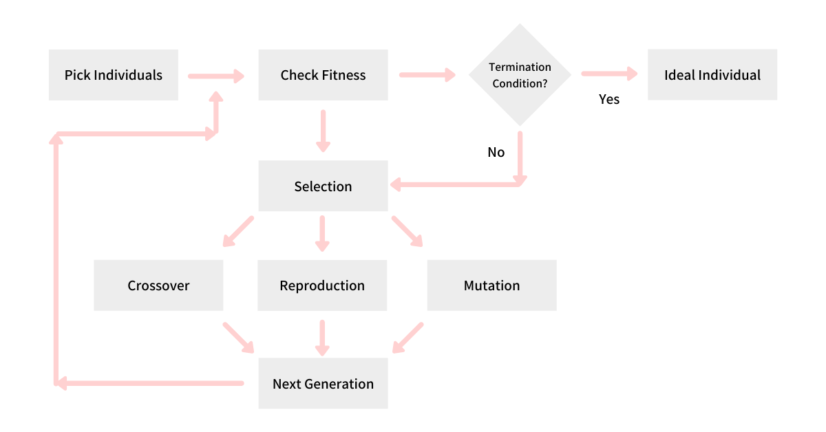
Creating one generation after another continues until we hit a termination condition. Post which the fittest solution is our high-quality solution to the problem. We take the example of the Knapsack problem and try to solve it using a Genetic Algorithm.

Knapsack using Genetic Algorithm

Say, we have a knapsack that can hold 15kg of weight at max. We have 4 items A, B, C, and D; having weights of 7kg, 2kg, 1kg, and 9kg; and value $5, $4, $7, and $2 respectively. Let’s see how we can find a high-quality solution to this Knapsack problem using a Genetic Algorithm and, in the process, understand each step of it.

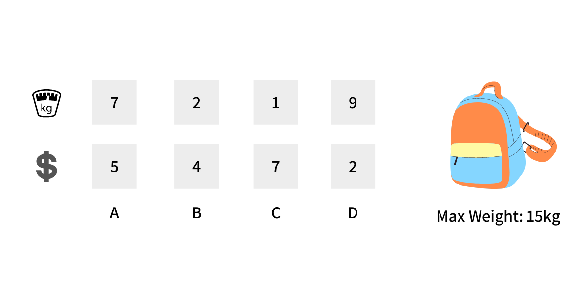
The above example is taken from the Computerphile’s video on this same topic.

Individual Representation

An Individual in the Genetic Algorithm is a potential solution. We first find a way to represent it such that it allows us to evolve. For our knapsack problem, this representation is pretty simple and straightforward; every individual is an n-bit string where each bit correspond to an item from the n items we have.

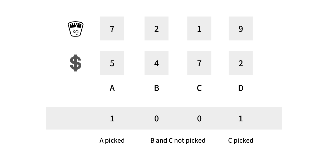
Given that we have 4 items, every individual will be represented by a 4-bit string and the ith position in this string will denote if we picked that item in our knapsack or not, depending on if the bit is 1 or 0 respectively.

Picking Individuals

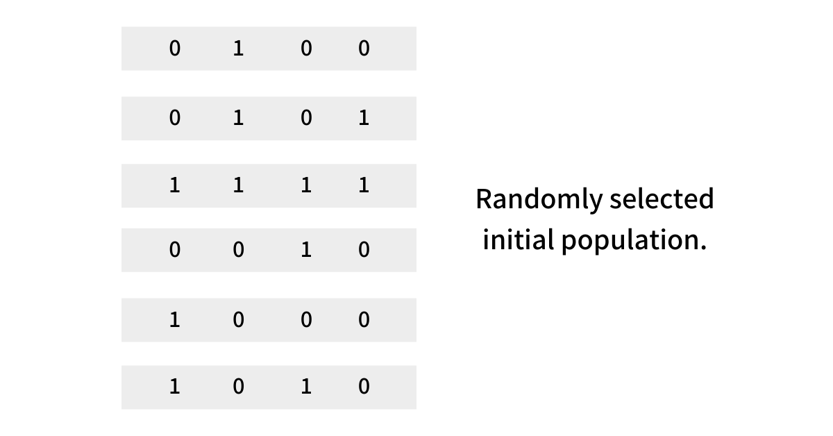
Now that we have our Individual representation done, we pick a random set of Individuals that would form our initial population. Every single individual is a potential solution to the problem. Hence for the Knapsack problem, from a search space of 2^n, we pick a few individuals randomly.

The idea here is to evolve the population and make them fitter over time. Given that the search space is exponential, we use evolution to quickly converge to a high-quality (need not be optimal) solution. For our knapsack problem at hand, let us start with the following 6 individuals (potential solutions) as our initial population.

def generate_initial_population(count=6) -> List[Individual]:
    population = set()

    # generate initial population having `count` individuals
    while len(population) != count:
        # pick random bits one for each item and
        # create an individual
        bits = [
            random.choice([0, 1])
            for _ in items
        ]
        population.add(Individual(bits))

    return list(population)

Fitness Coefficient

Now that we have our initial population randomly chosen, we define a fitness coefficient that would tell us how fit an individual from the population is. The fitness coefficient of an individual totally depends on the problem at hand, and if implemented poorly or incorrectly, it can result in misleading data or inefficiencies. The value of the fitness coefficient typically lies in the range of 0 to 1. but not a mandate.

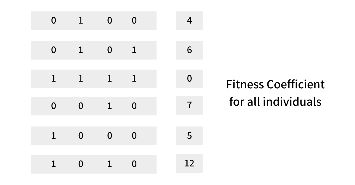
For our knapsack problem, we can define the fitness coefficient of an individual (solution) as the summation of the values of the items picked in the knapsack as per the bit string if the total weight of the picked items is less than the weight knapsack can hold. The fitness coefficient of an individual is 0 if the total weight of the item picked is greater than the weight that the knapsack can hold.

For the bit string 1001 the fitness coefficient will be

total_value  = (1 * v(A)) + (0 * v(B)) + (0 * v(C)) + (1 * v(D))
             = ((1 * 5) + (0 * 4) + (0 * 7) + (1 * 2))
	         = 5 + 0 + 0 + 2
	         = 7

total_weight = (1 * w(A)) + (0 * w(B)) + (0 * w(C)) + (1 * w(D))
             = ((1 * 7) + (0 * 2) + (0 * 1) + (1 * 9))
	         = 7 + 0 + 0 + 9
	         = 16

Since, MAX_KNAPSACK_WEIGHT is 15
the fitness coefficient of 1001 will be 0

The higher the individual’s fitness, the more are the chances of that individual to move forward as part of the evolution. This is based on a very common evolutionary concept called Survival of the Fittest.

def fitness(self) -> float:
    total_value = sum([
        bit * item.value
        for item, bit in zip(items, self.bits)
    ])

    total_weight = sum([
        bit * item.weight
        for item, bit in zip(items, self.bits)
    ])

    if total_weight <= MAX_KNAPSACK_WEIGHT:
        return total_value

    return 0

Selection

Now that we have defined the Fitness Coefficient, it is time to select a few individuals to create the next generation. The selection happens using selection criteria inspired by evolutionary behavior. This is a tunable parameter we pick and experiment with while solving a particular problem.

One good selection criteria is Tournament Selection, which randomly picks two individuals and runs a virtual tournament. The one having the higher fitness coefficient wins.

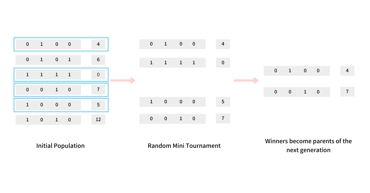
For our knapsack example, we randomly pick two individuals from the initial population and run a tournament between them. The one who wins becomes the first parent. We repeat the same procedure and get the second parent for the next step. The two parents are then passed onto the next steps of evolution.

def selection(population: List[Individual]) -> List[Individual]:
    parents = []

    # randomly shuffle the population
    random.shuffle(population)

    # we use the first 4 individuals
    # run a tournament between them and
    # get two fit parents for the next steps of evolution

    # tournament between first and second
    if population[0].fitness() > population[1].fitness():
        parents.append(population[0])
    else:
        parents.append(population[1])

    # tournament between third and fourth
    if population[2].fitness() > population[3].fitness():
        parents.append(population[2])
    else:
        parents.append(population[3])

    return parents

Crossover

Crossover is an evolutionary operation between two individuals, and it generates children having some parts from each parent. There are different crossover techniques that we can use: single-point crossover, two-point crossover, multi-point crossover, uniform crossover, and arithmetic crossover. Again, this is just a guideline, and we are allowed to choose the crossover function and the number of children to create we desire.

The crossover does not always happen in nature; hence we define a parameter called the Crossover Rate, which is relatively in the range of 0.4 to 0.6 given that in nature, we see a similar rate of crossover while creating offspring.

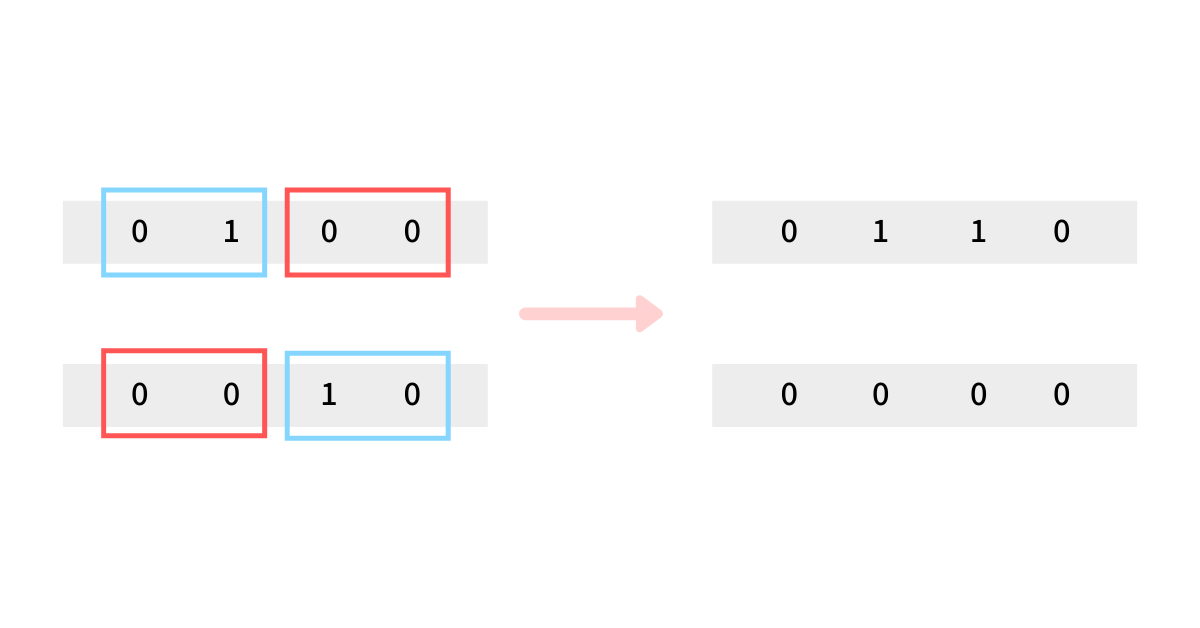
For our knapsack problem, we keep it simple and create two children from two fit parents such that both get one half from each parent and the other half from the other parent. This essentially means that we combine half elements from both the individual and form the two children.

def crossover(parents: List[Individual]) -> List[Individual]:
    N = len(items)

    child1 = parents[0].bits[:N//2] + parents[1].bits[N//2:]
    child2 = parents[0].bits[N//2:] + parents[1].bits[:N//2]

    return [Individual(child1), Individual(child2)]

Mutation

The mutation is an evolutionary operation that randomly mutates an individual. This is inspired by the mutation that happens in nature, and the core idea is that sometimes you get some random unexpected changes in an individual.

Just like the crossover operation, the mutation does not always happen. Hence, we define a parameter called the Mutation Rate, which is very low given that mutation rate in nature. The rate typically is in the range of 0.01 to 0.02. The mutation changes an individual, and with this change, it can have a higher or lower fitness coefficient, just how it happens in nature.

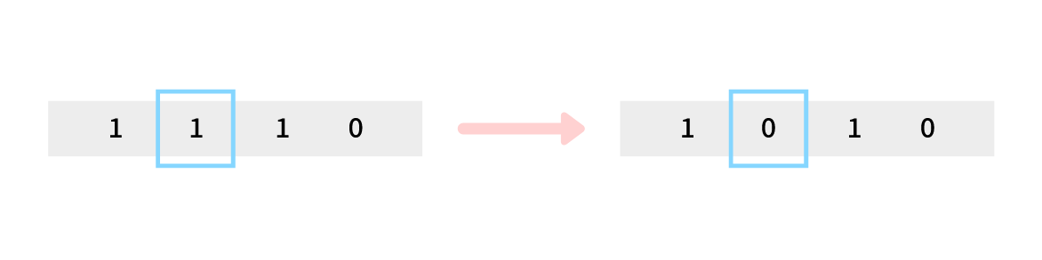
For our knapsack problem, we define a mutation rate and choose to flip bits of the children. Our mutate function iterates through the bits and sees if it needs to flip as per the mutation rate. If it needs to, then we flip the bit.

def mutate(individuals: List[Individual]) -> List[Individual]:
    for individual in individuals:
        for i in range(len(individual.bits)):
            if random.random() < MUTATION_RATE:
                # Flip the bit
                individual.bits[i] = ~individual.bits[i]

Reproduction

Reproduction is a process of passing an individual as-is from one generation to another without any mutation or crossover. This is inspired by nature, where evolutionary there is a very high chance that the genes of the fittest individuals are passed as is to the next generation. By passing the fittest individuals to the next generation, we get closer to reaching the overall fittest individual and thus the optimal solution to the problem.

Like what we did with the Crossover and the Mutation, we define a Reproduction Rate. Upon hitting that, the two fittest individuals will not undergo any crossover or mutation; instead, they would be directly passed down to the next generation.

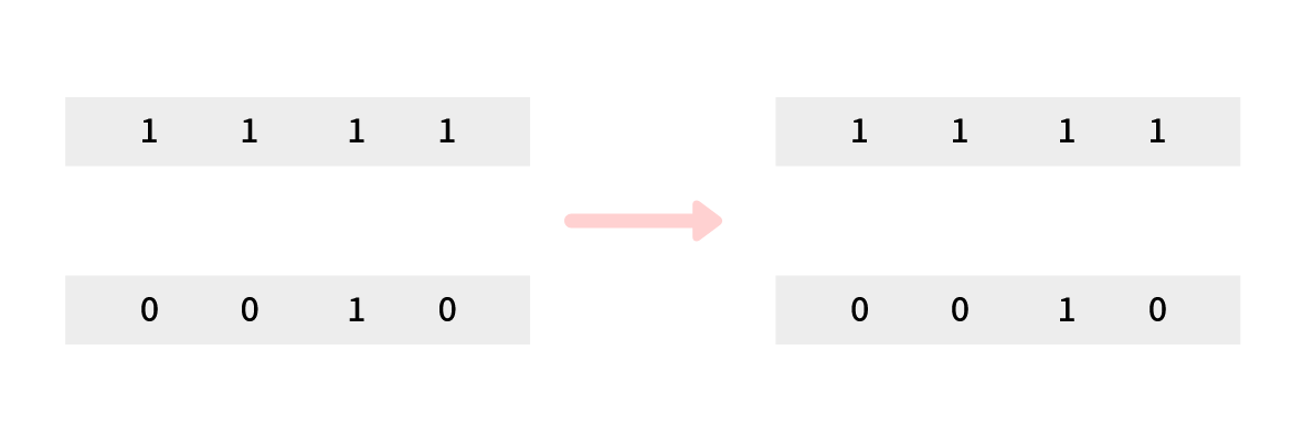
For our knapsack problem, we define a Reproduction Rate and, depending on what we decide to pass the fittest individuals to the next generation directly. We keep the reproduction rate to 0.30 implying that 30% of the time, the fittest parents are passed down as is to the next generation.

Creating Generations

We repeat the entire process of Selection, Reproduction, Crossover, and Mutation till we get the same number of children as the initial population, and we call it the first generation. We repeat the same process again and create subsequent generations.

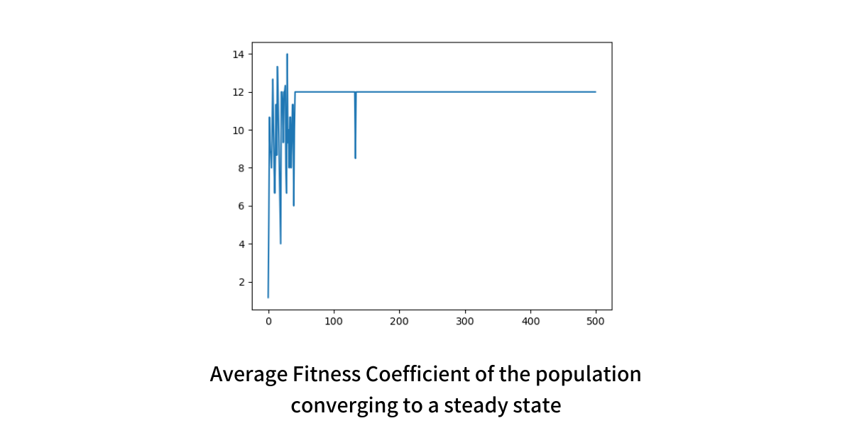
When we continue to create such generations, we will observe that the Average Fitness Coefficient of the population increases and it converges to a steady range. The image above shows how our value converges to 12 over 500 generations for the given problem. The optimal solution to the problem at hand is 16, and we converged to 12.

def next_generation(population: List[Individual]) -> List[Individual]:
    next_gen = []
    while len(next_gen) < len(population):
        children = []

        # we run selection and get parents
        parents = selection(population)

        # reproduction
        if random.random() < REPRODUCTION_RATE:
            children = parents
        else:
            # crossover
            if random.random() < CROSSOVER_RATE:
                children = crossover(parents)

            # mutation
            if random.random() < MUTATION_RATE:
                mutate(children)

        next_gen.extend(children)

    return next_gen[:len(population)]

Termination Condition

We can continue to generate generations upon generations in search of the optimal solution, but we cannot go indefinitely, which is where we need a termination condition. A good termination condition is deterministic and capped. For example, we will at max go up to 500 or 1000 generations or until we get the same Average Fitness Coefficient for the last 50 values.

We can have a similar terminating condition for our knapsack problem where we put a cap at 500 generations. The individual with the max fitness coefficient is our high-quality solution. The overall flow looks something like this.

def solve_knapsack() -> Individual:
    population = generate_initial_population()

    avg_fitnesses = []

    for _ in range(500):
        avg_fitnesses.append(average_fitness(population))
        population = next_generation(population)

    population = sorted(population, key=lambda i: i.fitness(), reverse=True)
    return population[0]

Run-time Complexity

The run-time complexity of the Genetic Algorithm to generate a high-quality solution for the Knapsack problem is not exponential, but it is polynomial. If we operate with the population size of PAnd iterate till G generations, and F is the run-time complexity of the fitness function, the overall complexity of the algorithm will be O(P.G.F).

Given that the parameters are known before starting the execution, you can predict the time taken to reach the solution. Thus, we are finding a non-optimal but high-quality solution to the infamous Knapsack problem in Polynomial Time.

Multi-dimensional optimization problems

The problem we discussed was trivial and was enough for us to understand the core idea of the Genetic Algorithm. The true power of the Genetic Algorithm comes into action when we have multiple parameters, dimensions, and constraints. For example, instead of just weight what if we have size and fragility as two other parameters to consider and we have to find a high-quality solution for the same Knapsack problem.

The efficiency of Genetic Algorithm

While discussing the process of Genetic Algorithm, we saw that there are multiple parameters that can increase or decrease the efficiency of the algorithm; a few factors include

Population

The size of the initial population is critical in achieving the high efficiency of a Genetic Algorithm. For our Knapsack problem, we started with a simpler problem with 4 items i.e. search space of a mere 16, and an initial population of 6. We took such a small problem set just to wrap our heads around the idea.

In the real-world, genetic algorithms operate on a much larger search space and typically start with a population size of 500 to 50000. It is observed that if the initial population size does not affect the execution time of the algorithm, it converges faster with a large population than a smaller one.

Crossover

As we discussed above there are multiple Crossover functions that we can use, like Single Point Crossover, Two-point Crossover, and Multi-point Crossover. Which crossover function would work better for a problem depends totally on the problem at hand. It is generally observed that the two-point crossover results in the fastest convergence.

You can find the complete source code to the genetic algorithm discussed above in the repository github/genetic-knapsack