Introduction

Singular Value Decomposition (SVD) is a powerful matrix factorization technique widely used in various fields, including machine learning, data compression, and signal processing. However, performing SVD on large matrices can be computationally expensive. Randomized SVD is an efficient algorithm that approximates the SVD of large matrices using random projections.

In this blog post, I would like to quickly discuss the mathematical motivations behind Randomized SVD and outline the algorithm.

Prerequisites

Orthonormal Columns

Suppose $Q$ is a matrix with orthonormal columns, then we have $Q^{\top} Q = I$.

Orthonormal Projection

Suppose $Q$ is a matrix with orthonormal columns of shape $m \times k$, then the matrix $P = Q Q^{\top}$ is an orthonormal projection matrix projecting onto the column space of $Q$. For any vector $x$ of shape $m \times 1$, the projection of $x$ onto the column space of $Q$ is given by $P x = Q Q^{\top} x$. The matrix $P$ is symmetric and idempotent, i.e., $P^{\top} = P$ and $P^2 = P$.

Note that $Q Q^{\top} x$ is different from $Q^{\top} x$. $Q^{\top} x$ gives the coordinates of $x$ in the basis formed by the columns of $Q$, while $Q Q^{\top} x$ is the point that is the closest to $x$ in the column space of $Q$, i.e., the orthonormal projection of $x$ onto the column space of $Q$.

For example, suppose we have a point $x = [1, 1]$ and a matrix that only consists of one orthonormal column.

$$
Q = \begin{bmatrix}
1 \\
0
\end{bmatrix}
$$

The coordinates of $x$ in the basis formed by the column of $Q$ is given by:

$$
Q^{\top} x = \begin{bmatrix}
1 & 0
\end{bmatrix}
\begin{bmatrix}
1 \\
1
\end{bmatrix}
= 1
$$

The point that is the closest to $x$ in the column space of $Q$ is given by:

$$
Q Q^{\top} x = \begin{bmatrix}
1 \\
0
\end{bmatrix}
\begin{bmatrix}
1 & 0
\end{bmatrix}
\begin{bmatrix}
1 \\
1
\end{bmatrix}
= \begin{bmatrix}
1 \\
0
\end{bmatrix}
$$

The closest point to $x$ in the column space of $Q$ is $Q Q^{\top} x = [1, 0]$. We could not find any other point in the column space of $Q$ that is closer to $x$ than $[1, 0]$.

This can also be proved mathematically.

Proof

Let $y = Q c$ be any point in the column space of $Q$, where $c$ is a vector of shape $k \times 1$. The squared distance between $x$ and $y$ is given by:

$$
| x - y |^2 = | x - Q c |^2
$$

The squared distance between $x$ and $y$ is minimized when $c = Q^{\top} x$:

$$
\begin{aligned}
| x - Q c |^2 &= (x - Q c)^{\top} (x - Q c) \\
&= x^{\top} x - 2 c^{\top} Q^{\top} x + c^{\top} c
\end{aligned}
$$

The squared distance is minimized when the derivative with respect to $c$ is zero:

$$
\frac{\partial}{\partial c} | x - Q c |^2
= -2 Q^{\top} x + 2 c = 0
$$

Solving for $c$ gives:

$$
c = Q^{\top} x
$$

The squared distance between $x$ and $y$ is then given by:

$$
\begin{aligned}
| x - y |^2 &= | x - Q c |^2 \\
&= | x - Q Q^{\top} x |^2 \\
&= | (I - Q Q^{\top}) x |^2
\end{aligned}
$$

This concludes the proof. $\square$

If $x$ is already in the column space of $Q$, then $(I - Q Q^{\top}) x = 0$ and the squared distance is exactly zero. In this case, $x = Q c$ for some $c$ and the projection of $x$ onto the column space of $Q$ is $Q Q^{\top} x = Q Q^{\top} Q c = Q \left(Q^{\top} Q\right) c = Q I c = Q c = x$. So the distance between $x$ and its projection $Q Q^{\top} x$ is zero.

So if the column space of $Q$ captures most of the “energy” of the data points, then the projection of the data points onto the column space of $Q$ will be very close to the original data points.

Suppose $A$ is a data matrix of shape $m \times n$, without loss of generality, we could assume that $m \geq n$, and $A$ has rank $d$, $m \geq n \geq d$. If we could find a matrix $Q$ of shape $m \times k$ with orthonormal columns, where $k \leq d$, such that the column space of $Q$ captures most of the “energy” of the data points in $A$, then we could use $Q Q^{\top} A$ to approximate $A$ with a lower-rank matrix $Q$.

QR Decomposition

QR decomposition is a matrix factorization technique that decomposes a matrix $A$ of shape $m \times n$ into the product of an orthogonal matrix $Q$ and an upper triangular matrix $R$. The QR decomposition of a matrix $A$ is given by:

$$
A = QR
$$

where $Q$ is an orthogonal matrix of shape $m \times m$, and $R$ is an upper triangular matrix of shape $m \times n$. The QR decomposition can be computed using various algorithms, such as the Gram-Schmidt process or the Householder reflections.

If $A$ is lower rank, we could use the thin QR decomposition to get $Q$ with orthonormal columns. The thin QR decomposition of a matrix $A$ of shape $m \times n$ with rank $d$ is given by:

$$
A = QR
$$

where $Q$ is of shape $m \times d$ with orthonormal columns, and $R$ is of shape $d \times n$.

Singular Value Decomposition (SVD)

Singular Value Decomposition (SVD) is a matrix factorization technique that decomposes a matrix $A$ of shape $m \times n$ into the product of three matrices: $U$, $\Sigma$, and $V^{\top}$. The SVD of a matrix $A$ is given by:

$$
A = U \Sigma V^{\top}
$$

where $U$ is an orthogonal matrix of shape $m \times m$, $\Sigma$ is a diagonal matrix of shape $m \times n$ with non-negative singular values on the diagonal, and $V$ is an orthogonal matrix of shape $n \times n$.

If $A$ has rank $d$, then only the first $d$ singular values in $\Sigma$ are non-zero. We could use the compact SVD to get a more compact representation of $A$. The compact SVD of a matrix $A$ of shape $m \times n$ with rank $d$ is given by:

$$
A = U \Sigma V^{\top}
$$

where $U$ is of shape $m \times d$, $\Sigma$ is of shape $d \times d$, and $V$ is of shape $n \times d$.

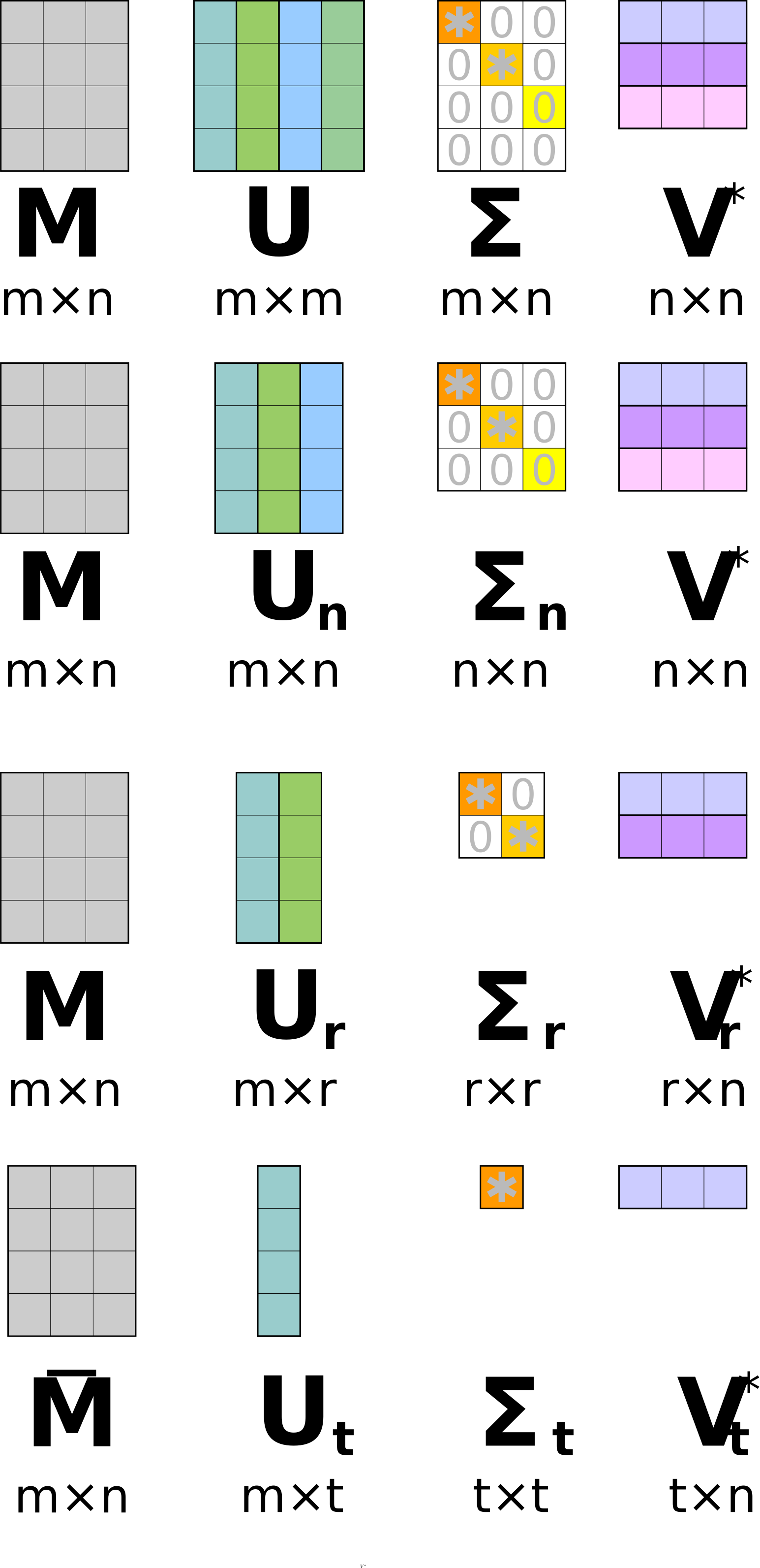
If we only keep the top $k$ singular values and their corresponding singular vectors, where $k \leq d$, we could get the rank-$k$ approximation of $A$ as follows:

$$
A \approx U_k \Sigma_k V_k^{\top}
$$

where $U_k$ is of shape $m \times k$, $\Sigma_k$ is of shape $k \times k$, and $V_k$ is of shape $n \times k$.

SVD is useful for data compression, which reduces the storage requirement for large data matrix $A$ from $\mathcal{\Theta}(mn)$ to $\mathcal{\Theta}(k(m+n+k))$, where $k$ is the target rank. When $k \ll \min(m, n)$, the storage saving could be significant.

Randomized SVD

Performing SVD on the large data matrix $A$ directly could be computationally expensive. Instead, if we know the orthonormal basis $Q$ that captures most of the “energy” of the data points in $A$, we could first project $A$ onto the column space of $Q$ to get a smaller matrix $B = Q^{\top} A$ of shape $k \times n$, then perform SVD on the smaller matrix $B$ to get its SVD decomposition $B = \tilde{U} \Sigma V^{\top}$, where $\tilde{U}$ is of shape $k \times k$, $\Sigma$ is of shape $k \times n$, and $V$ is of shape $n \times n$. Finally, we could reconstruct the approximate SVD decomposition of $A$ as follows:

$$
\begin{align}
A
&\approx Q Q^{\top} A \\
&= Q B \\
&= Q \tilde{U} \Sigma V^{\top} \\
&= U \Sigma V^{\top}
\end{align}
$$

where $U = Q \tilde{U}$ is of shape $m \times k$.

So the question is how to find the orthonormal basis $Q$ that captures most of the “energy” of the data points in $A$ efficiently. Certainly we could use QR decomposition on $A$ directly to get $Q$, but this could still be computationally expensive for large matrices.

If we could reduce the size of $A$ from $m \times n$ to $m \times r$ while still preserving the orthonormal basis of the column space of $A$, where $r$ is slightly larger than $k$, then we could perform QR decomposition on the smaller matrix to get $Q$ efficiently. This is where random projection comes in.

The hypothesis is that if we project the data points in $A$ onto a random subspace of dimension $r$ using some random matrix $P$ of shape $n \times r$, when $r$ is slightly larger than $k$, the rank of $A$, with high probability, the orthonormal basis of the column space of the projected data points will be very close to the orthonormal basis of the column space of the original data points. This matrix $P$ cannot be any arbitrary matrix. For example, if $P$ is a matrix of all zeros, then the projected data points will all be zero and we cannot recover any information about the original data points. A common choice of $P$ is a Gaussian random matrix, where each entry is sampled from a standard normal distribution. Once we have the shrunken data matrix $Z = A P$ of shape $m \times r$, we could perform QR decomposition on $Z$ to get $Q$ of shape $m \times r$ with orthonormal columns. Then we could proceed with the steps mentioned above to compute the approximate SVD decomposition of $A$.

Concretely, the steps of the randomized SVD algorithm are as follows:

1. Generate a Gaussian random matrix $P$ of shape $n \times r$. When $r$ is smaller than the rank of matrix $A$, $k$, there starts to be information loss.
2. Compute the shrunken data matrix $Z = A P$ of shape $m \times r$.
3. Perform QR decomposition on $Z$ to get $Q$ of shape $m \times r$ with orthonormal columns.
4. Compute the smaller matrix $B = Q^{\top} A$ of shape $r \times n$.
5. Perform SVD on $B$ to get $B = \tilde{U} \Sigma V^{\top}$.
6. Compute $U = Q \tilde{U}$ of shape $m \times r$.
7. The approximate SVD decomposition of $A$ is given by $A \approx U \Sigma V^{\top}$.

References

• Randomized Singular Value Decomposition
• Randomized SVD
• A Systematic Review of Low-Rank and Local Low-Rank Matrix Approximation In Big Data Medical Imaging
• Singular Value Decomposition - Wikipedia