here’s my final hackathon of the year (2024). there are a few concepts in deep learning that i simply love. they include (but are not limited to) autoregressive sequence modeling, mixture density networks, boltzmann machines, variational autoencoders, stochastic gradient descent with adaptive learning rate and more recently set transformers. so, as the final hackathon of this year, i’ve decided to see if i can put together a set transformer, an autoregressive transformer decoder and a mixture density network to learn to infer an underlying mixture of Gaussians. i’ve got some help (and also misleading guidances) from Google Gemini (gemini-exp-1206) , which was overall positive, since i was able to put together the whole thing in about two days (and two extra days for me to figure out the issue of layernorm). so, here you go:

This post explores a proof of concept for “learning to X” by designing and implementing an Amortized Mixture of Gaussians (AMoG). The core idea is to train a neural network to analyze samples from an unknown mixture of Gaussians and predict its components. This network is trained on numerous synthetic examples, each comprising:

1. A randomly generated Mixture of Gaussians (MoG): \( \left\{ (\mu_k, \sigma_k^2) \right\}_{k=1}^K \)
2. Samples drawn from this MoG: \( D=\left\{ x_n \right\}_{n=1}^N \)

For simplicity, we assume equal component likelihoods and diagonal covariance for each component.

The neural network’s task is to map \( \left\{x_n\right\}_{n=1}^N \) to \( \left\{ (\mu_k, \sigma_k^2) \right\}_{k=1}^K \), where \(N\) and \(K\) can vary. This has two possible interpretations:

1. The network outputs a MoG closely fitting the input data.
2. The network outputs the parameters of the original MoG that generated the data.

This post focuses on (2), recovering the original parameters, which is feasible due to the synthetic dataset.

Model Architecture: A Set-Conditioned Autoregressive Model with a Mixture Density Network Head

We construct a neural network that sequentially outputs one component at a time, given the sample set. At each step, we determine component existence:

\[ p(e_k = 1 | e_{ < k}, \mu_{ < k}, \log \sigma_{ < k}, D) = \mathrm{sigmoid}(w_e^\top h_k + b_e) \]

where \(h_k\) is the \(k\)-th hidden state from an autoregressive transformer:

\[ h_k = \mathrm{transformer}(([z, e_1, \mu_1, \log \sigma_1], \ldots, [z, e_{k-1}, \mu_{k-1}, \log \sigma_{k-1}])) \]

\(z\) is the output from a set transformer:

\[ z = \mathrm{setTransformer}(\left\{ x_n \right\}_{n=1}^N) \]

For the mean and variance of the \(k\)-th component, the network outputs a mixture of Gaussians, similar to mixture density networks, to handle component ordering uncertainty:

\[ p(\mu_k = \mu | e_{ < k}, \mu_{ < k}, \log \sigma_{ < k}, D) = \sum_{m=1}^M \alpha_\mu^m \mathcal{N}(\mu | v_\mu^m, s_\mu^m) \]

\[ p(\log \sigma_k = s | e_{ < k}, \mu_{ < k}, \log \sigma_{ < k}, D) = \sum_{m=1}^M \alpha_\sigma^m \mathcal{N}(s | v_\sigma^m, s_\sigma^m) \]

where \(\alpha_\mu^m\), \(v_\mu^m\), \(s_\mu^m\), \(\alpha_\sigma^m\), \(v_\sigma^m\), and \(s_{\sigma}^m\) are derived from \(h_k\). The coefficients \(\alpha_\cdot^m\) sum to 1 via softmax. This mixture density network approach is crucial due to the lack of inherent ordering in MoG components.

We won’t delve into the specifics of \(\mathrm{Transformer}\) and \(\mathrm{setTransformer}\) implementations, as they follow standard practices. The code is available at https://github.com/kyunghyuncho/amortized-mog. (Please excuse the messy commit history – it reflects some initial misdirection by Google Gemini related to layer normalization.)

Training the Network

We employ maximum likelihood learning to train the entire network end-to-end:

\[
\begin{aligned}
& \sum_{\{((e_{k’}, \mu_{k’}, \log \sigma_{k’}))_{k’=1}^K, D\} \in \mathrm{data}} \sum_{k=1}^{K_\max} \log p(e_k = I(k \leq K) | e_{ < k}, \mu_{ < k}, \log \sigma_{ < k}, D) \\ & \qquad\qquad + I(k \leq K) ( \log p(\mu_{k} | e_{ < k}, \mu_{ < k}, \log \sigma_{ < k}, D) + \log p(\log \sigma_{k} | e_{ < k}, \mu_{ < k}, \log \sigma_{ < k}, D) ), \end{aligned} \]

where \(K_\max\) is the maximum number of components. This can be a large number or the maximum within the training set (or minibatch).

\(I(a)\) is an indicator function, returning 1 if \(a\) is true, 0 otherwise. Component parameters are used only when \(e_k = 1\). The component existence classifier is trained beyond the number of components, enabling the model to determine when to stop.

The network, comprising \(\mathrm{Transformer}\) and \(\mathrm{setTransformer}\), is trained jointly to maximize the objective function \(J\). We use minibatch learning with Adam as the optimizer.

Inference: Greedy Decoding

Finding the most likely MoG is intractable. Instead, we use greedy decoding, extracting one component at a time:

\[ \hat{e}_k = \arg\max_{e \in \{0, 1\}} \log p(e_k = e | e_{ < k}, \mu_{ < k}, \log \sigma_{ < k}, D) \]

If \(\hat{e}_k = 0\), we terminate. Otherwise,

\[ \hat{\mu}_k = v_{\mu}^{\hat{m}} \quad\text{and}\quad \log \hat{\sigma}_k = v_{\sigma}^{\hat{m}’} \]

where

\[ \begin{aligned} &\hat{m} = \arg\max_{m \in \{1, \ldots, M\}} \alpha_{\mu}^m \\ &\hat{m}’ = \arg\max_{m \in \{1, \ldots, M\}} \alpha_{\sigma}^m \end{aligned} \]

This is suboptimal but tractable. Potential improvements include gradient-based optimization to find the mode of the mixture density network and beam search instead of greedy decoding. These are left for future exploration.

Qualitative Analysis

Training Setup

We implemented the amortized MoG using PyTorch and PyTorch Lightning. For comparison, we use scikit-learn‘s GaussianMixture, which employs the Expectation-Maximization (EM) algorithm. In our simple 2D case, EM is expected to be near-optimal, serving as an oracle rather than a baseline. We provide GaussianMixture with the true number of components.

The amortized MoG is trained on an infinite stream of 100-sample datasets, each from a random mixture of at most five Gaussians. Components are separated by at least 2 (in mean distance). Covariance is diagonal with values between \(e^{-2}\) and \(e^{2}\). We reserve 500 examples as a validation set to monitor generalization. Training stops when validation loss plateaus.

Important Implementation Note: Layer normalization, common in transformers, can be detrimental with permutation invariance. It preserves relative positions but discards original coordinate information, crucial for the amortized MoG. Thus, layer normalization is disabled in setTransformer.

Case Studies

Instead of rigorous evaluation, we present three illustrative cases:

Case 1: Well-Separated Gaussian Components

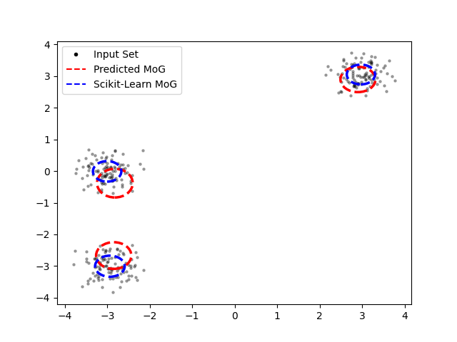
The amortized MoG performs well, accurately identifying the number of components and their clusters, although with slight offsets in the centers of the two left-side clusters.

Case 2: Gaussian and Uniform Components

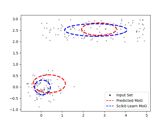
Here, one component is a uniform distribution over a rectangular region. The amortized MoG successfully identifies both well-separated components. Though, it is clear that the amortized MoG network is struggling to get the covariance correct. This may simply be due to the insufficient representational power of the neural network used in this experiment.

Case 3: Overlapping Components

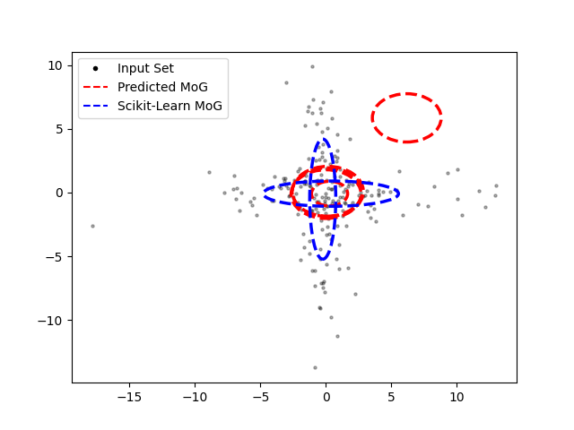
This challenging case features two overlapping components, one elongated horizontally and the other vertically. EM, with the known number of components, performs well. The amortized MoG struggles, predicting five components (the maximum allowed) concentrated around the origin. This highlights the importance of a well-designed data generating process for robust amortized inference.

Limitations and Future Work

Traditional methods for fitting MoGs are stochastic variational inference and EM. The proposed approach implicitly approximates these or potentially discovers a novel method. These algorithms are iterative and complex, demanding a powerful neural network for even a rough approximation. However, increasing network power also increases computational cost, potentially negating the benefits.

A fundamental question is the motivation behind this approach. While established methods exist for MoG’s, they often struggle with models involving numerous discrete or combinatorial latent variables, leading to high variance due to sampling. The proposed approach, applicable to any probabilistic model with a random generation mechanism, seeks a solution that minimizes both variance and bias in such challenging scenarios. Furthermore, by using the proposed approach as an initializer to a more costly but unbiased inference algorithm, we may eentually end up with the best of both worlds.

This concept relates to simulation-based inference, or likelihood-free inference, where a neural network inverts a forward simulator (analogous to the probabilistic generating process). Simulation-based inference often involves approximating \(p(x|\theta)\) or \(p(\theta|x)\) for downstream inference. This note skips this intermediate step, directly targeting the final inference quantity.

In conclusion, this post demonstrates the potential of combining a set transformer, autoregressive transformer, and mixture density network as an effective inference engine. Future work will involve more rigorous evaluation on more complex problems.