As Chad mentioned in his post last week, we have been diving into what OpenAI is doing with WebRTC. Over the last months, we actually did a full teardown and compared OpenAI’s Realtime API to what powers chatgpt.com. What intrigued us most was how to measure response latency.

One of the key metrics for any voice bot is response latency – how quickly you can hear a response. If that metric is not below a certain threshold, even under bad network conditions, the conversation will not feel natural. The latency is not only dependent on how quickly the LLM can generate a response, but also how long it takes to get that response to the user. The latter part is the job of WebRTC. Together these give you a total response latency. We can measure the total latency from the raw RTP packets extracted from Chrome using the methodology described in this blog post about the video_replay tool. That approach works quite well to compare different services in a blackbox exploration too.

In this post, we review that methodology as applied to OpenAI’s Realtime API with WebRTC and analyze the results.

Note: the results shown here were obtained on January 4th, 2025. Results have improved since then, in particular when it came to the STUN roundtrip time.

STUN round trip time

Chrome’s webrtc-internals page, which we often use for analysis, excels at visualizing the results of the W3C getStats API. This visualization provides valuable information, such as the target bitrate and the number of bytes sent and received, offering additional insights into how OpenAI’s WebRTC API is configured.
For latency the STUN round trip time in the candidate-pair statistics reveals how long packets take to travel from client to server and back, representing the theoretical lower bound for response latency.

Typically, the round trip time (RTT) is around 60-70 ms here (which seems relatively high compared to other services), although two small bumps suggest possible packet loss. This can be reduced by deploying servers physically closer to users (which can be done e.g. using latency-based DNS such as Amazons route53).

The RTP packets and the response Latency

Next we analyze the extracted packets using Wireshark, a widely used network analyzer that excels at VoIP/WebRTC-specific tasks, such as packet filtering and even audio playback. By examining the resulting graphs, we can accurately estimate the system’s response latency.
You can download the PCAP we extracted here.

One bug stood out: all audio RTP packets sent by the other side include the RTP marker bit. In audio, this bit essentially instructs the jitter buffer to flush. Doing that on each packet makes no sense at all since it results in no buffer (and is not even how libWebRTC behaves):

Wireshark’s “RTP player” functionality (find it in the telephony section), proves highly useful for listening to Chrome-decrypted audio. We use this feature to investigate whether we can measure the response time.

It is relatively easy to determine when the actual speech from the server side starts as the silent content of the non-speech packets is always the same. Figuring out when Chad stopped speaking was a bit more complicated. One needs to replay the stream in Wireshark and pick a “silent” point in the waveform which allows going to the corresponding packet as shown below:

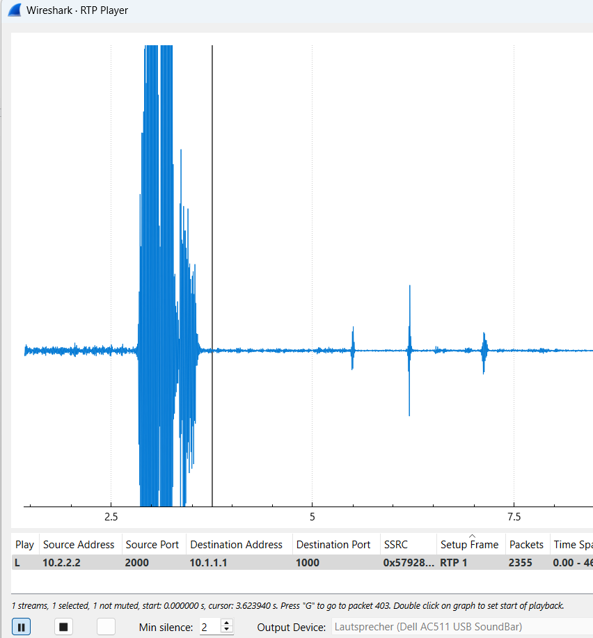
Marking the end of Chad’s speech (packet 403 in the screenshot) and the start of the model’s speech gives us a rough estimate of the response time:

End of speech packet/time	Start of response packet/time	Response delay
#399, 3.58s	#591, 5.27s	1.68s
#1335, 11.88s	#1535, 13.67s	1.78s
#2364, 21.10s	#2558, 22.77s	1.66s

That is obviously a very limited sample (and a very manual process), but the response delay is around 1.7 seconds.

Response latency measured with voice activity detection

libWebRTCs neteq_rtpplay tool, the audio equivalent of video_replay, can extract WAV files from the PCAP file with the unencrypted data.

This extracts the two RTP streams for caller and callee respectively. The packet starts are reasonably close together, 56 milliseconds as we can see in the PCAP using Wireshark:

Next, we import both WAV files into audacity, a versatile audio tool. It is easy to align both tracks based on the RTP offset mentioned earlier. The waveform also reveals a brief failure in echo cancellation on Chad’s end.

Now we will export the mix of both tracks as a single WAV file for easier playback. Now that we have an audio file, we need to identify the “speech” in it. For that, we can install silero-vad, a surprisingly common “AI” (or ML) based voice activity detection library to find the speech in a WAV file.

Next, we run the Python script below. It imports and initializes silero, loads the WAV file, and uses the helper function get_speech_timestamps to get an array of speech start and speech end timestamps. We dump those to timestamps in a similar format as the table above:

Running the script as python3 webrtchacks.py yields the following output:

While some of these speech events are false positives, we can see the three speaker switches with a gap of 1.764s, 1.86s, and 1.796s. There is a slight offset compared to the manually extracted values.

Measuring the response latency using the techniques shown is pretty accurate. While it ignores any delay created by playout, that is a constant offset. And the measurements can be automated fairly well.

Benchmarking as well as agreeing on how benchmarking is done is important.  Clearly there is some work left to do both for OpenAI – which really means Justin Uberti – as well as how WebRTC can be used for this use case. Stay tuned!

{
“author”: “Philipp Hancke“,
“editor”: “Chad Hart“,
“special-thanks”: “Justin Uberti”
}