With linear data structures like our array or linked list, navigating (aka traversing) through all of the items is fairly straightforward. We start at the beginning and just keep going to the next item until we hit the end, where there are no more items left:

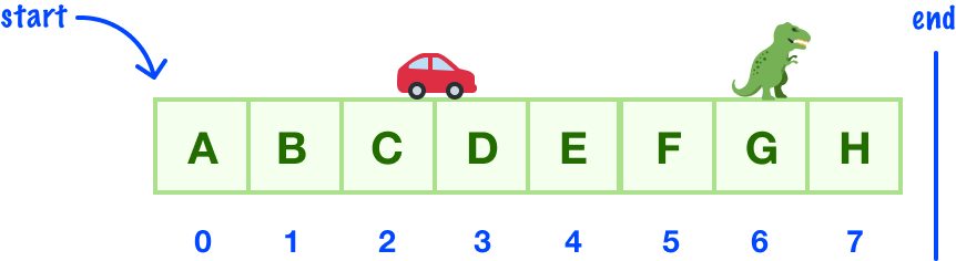
This nice and easy approach doesn’t work with trees:

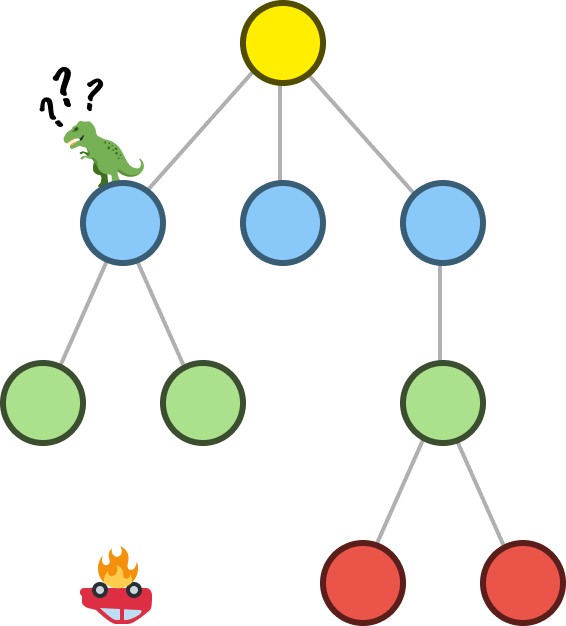
Trees are hierarchical data structures, so the way we traverse through them will need to be different. There are two types of traversal approaches we can use. One approach is breadth-first, and another approach is depth-first. In the following sections, we’ll go both broader and deeper (ha!) into what all of this means.

Onwards!

Breadth-First Traversal

Echoing a detail from when we first looked at trees, our trees have a depth or a level to them that indicates how far away they are from the root:

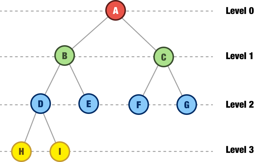
Level 0 (or Depth 0) is always going to be the root. All of the children nodes from there will find themselves on their own level depending on how far from the root they are.

In a breadth-first approach, these levels play an important role in how we traverse our tree. We traverse the tree level by level where we start from the root node and visit all the nodes at each level before moving on to the next level.

This will be clearer with an example. So, we start with our root node:

At this point, we don’t know much about our tree or what it looks like. The only thing we know is that we have a root node, so we explore it. We discover that our root node has two children, B and C:

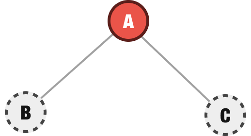
Here lies a subtle but important detail: Discovering is not the same thing as exploring. When we discover nodes, we are aware that they exist. When we explore them, we actively inspect them and see if they have any children or not. In our visualizations, when a node has simply been discovered, we'll display them in a dotted outline. Once a node has been explored, we'll display it in a solid outline.

From our discovered nodes B and C, we explore B first. It has two children:

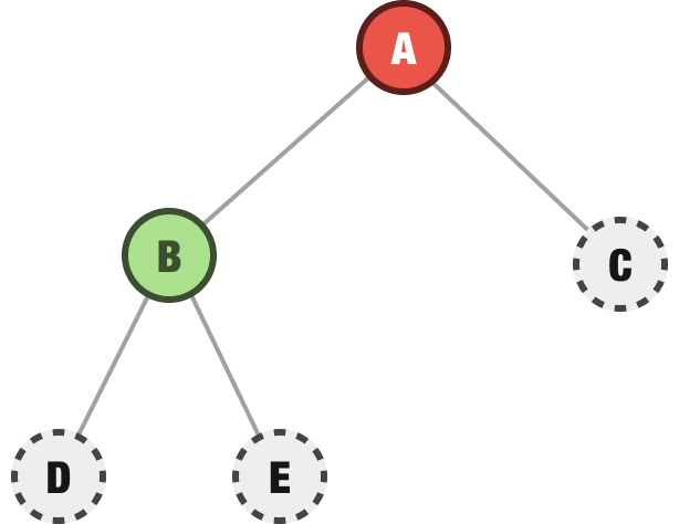
We ignore these newly discovered children for now. Instead, we continue on to exploring C and find out that it has two children as well:

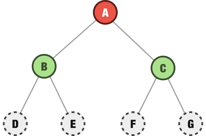
We are done with the current row made up of our B and C nodes, and we now repeat the process we’ve been following for the next row of nodes. We start on the left with the D node and explore it to see if it has any children. The D node does have two children:

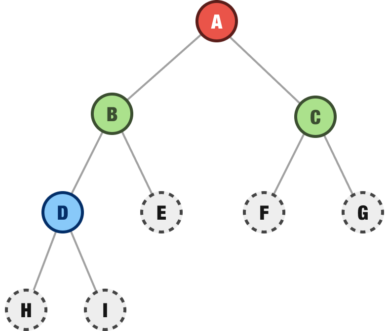
We then move on to the E node, the F node, and the G node and explore them to see if they have any children. They don't have any children:

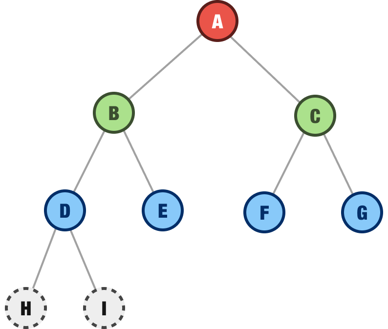
At this point, we are done exploring one more row. Now, it's time to go into the next row and see what is going on with the H and I nodes. The H node contains no children, and the I node contains no children as well. There are no more nodes to discover and explore, so we have reached the end of the line and have fully explored our tree:

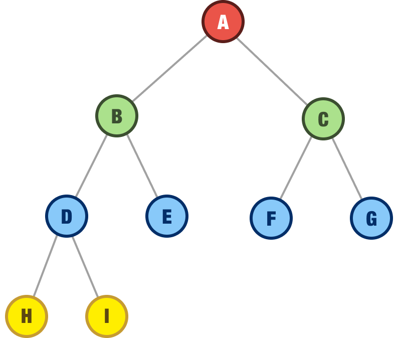
The order in which we explored our nodes is highlighted by the numbers in the following visualization:

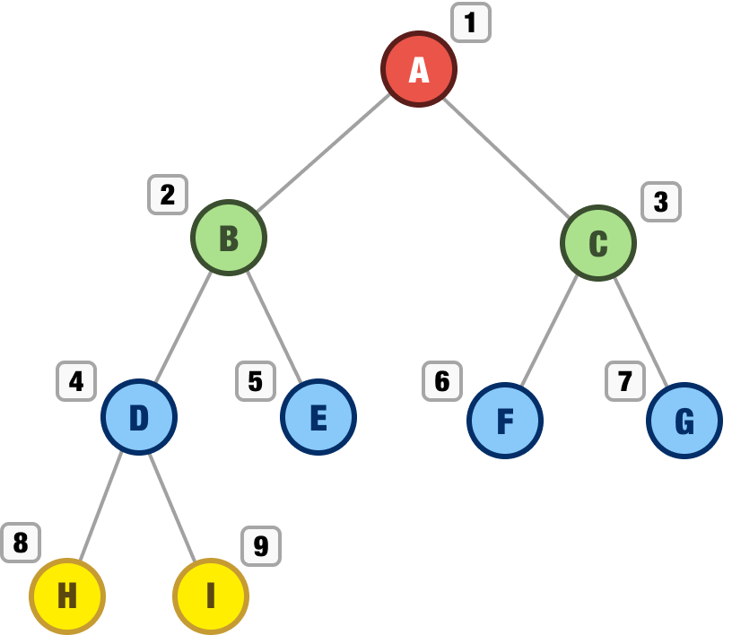
The order our nodes have been explored in is A, B, C, D, E, F, G, H, and I. The breadth first traversal approach is a bit like exploring a tree in a very organized and methodical way. This is quite a bit different than our next traversal approach...

Depth-First Traversal

The other popular way for traversing through our tree is the depth-first approach. Instead of exploring the tree level by level as we did with our breadth-first approach, in this depth-first world, we follow the left-most path as deeply as possible before backtracking and exploring another path.

Let’s walk through what this will look like. At the top, we have our root node:

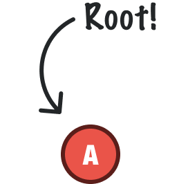
We explore it to see how many children it has, and we find out that it has two children, B and C:

Next, we are going to explore the B node and see if it has any children. As it turns out, we discover that it has two children:

Up until this point, what we have seen is consistent with the first few steps we took in our breadth-first approach earlier. Now, here is where things get different. Instead of exploring the C node next, we are instead going to go deeper into exploring B’s children, starting with the first left-most node. That would be the D node, so we explore it next:

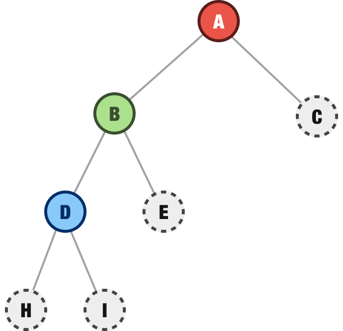
D’s children are H and I, but (under depth-first rules) we explore H next because it is the left-most first child node:

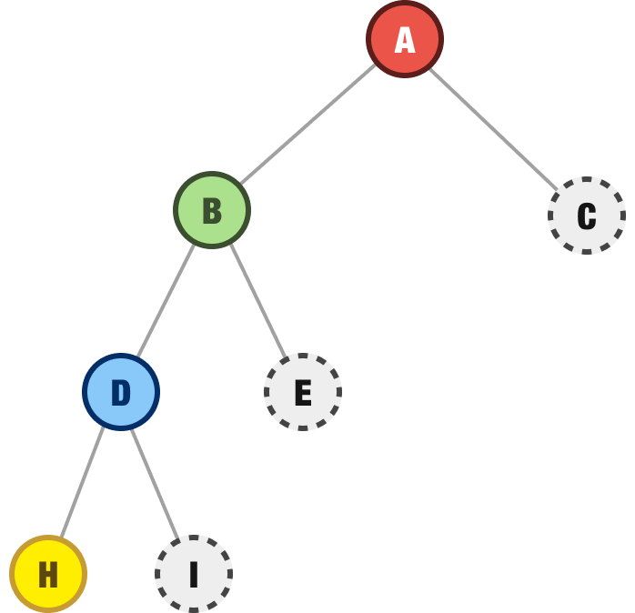
H does not have any children, so we then backtrack to the nearest unexplored node. This would be our I node:

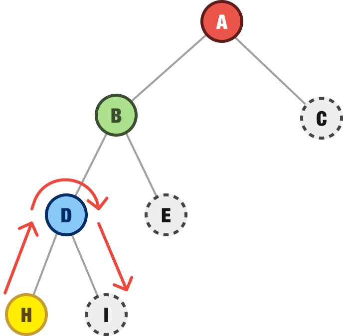
Our I node has no children either, so we backtrack even further to the next spot we have any unexplored children. That would be the E node:

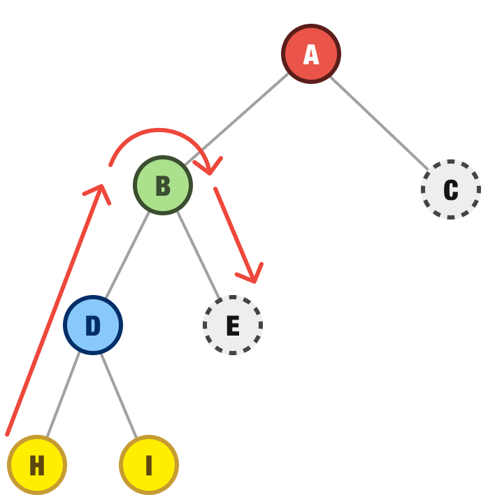
As it turns out, E has no child nodes so we continue on go to our next nearest destination where we have unexplored children. That would be the C node near the very top. When we explore the C node, we find it has two children - F and G:

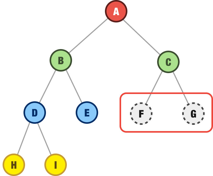
In classic depth-first fashion, we explore the F child node first. It has no children. We then backtrack to the next nearest unexplored node, which will happen to be G. It has no children as well, so we are now done exploring our tree:

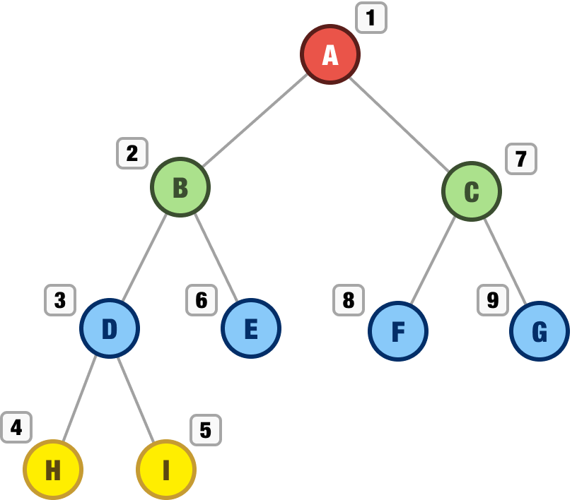
If we trace our steps, we did a lot of jumping around here. The order in which we explored our nodes is A, B, D, H, I, E, C, F, and G. We can visualize the order as follows:

To summarize the behavior we walked through in our dept-first approach, we explored:

1. Our root node first
2. The left subtree fully
3. The right subtree fully

There are several depth-first variations, and the three steps we saw here is referred to as a pre-order traversal. This is a popular variation we’ll be using for searching our tree later on, but other variations include post-order traversal and and in-order traversal. We will talk about those much later.

Implementing our Traversal Approaches

In the past few sections, we learned how both breadth-first and depth-first traversals work. It is now time for us to turn all of our knowledge into working code. As we will see in a few moments, the code for both breadth-first and depth-first traversals will look very similar to each other. There is a very good reason for this!

Backing up a bit, there are two steps to how a node gets explored:

1. Node is discovered. This is where we simply recognize that a node exists
2. Node is explored. This is where we examine the node and discover any children that we need to...um...discover.

Where both our traversal approaches vary is in how exactly our nodes get discovered, explored, and inserted. This is worth diving into, and we'll do that next.

Node Exploration in the Breadth-First Approach

Let’s say that we have a partially explored tree that looks as follows:

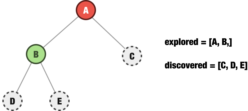
If we explicitly call out what we have explored and discovered, we’ll see that our explored nodes are A and B. Our discovered nodes are C, D, and E. It’s time to go exploring! In a breadth-first approach, the next node we explore is going to be the first item in our discovered collection of nodes. That would be node C, so let’s explore it next:

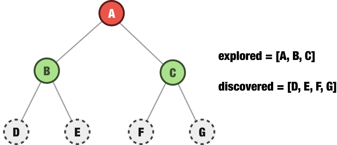
Notice what happened when we decided to explore node C. We removed C from our discovered collection and added it to the end of our explored collection. Node C has two children, F and G, so we added those to the end of our discovered collection for processing eventually. The rest of what happens follows this pattern. For our next step, we take the D node from the beginning of our discovered collection and add it to the end of our explored collection. If D happens to have any children that we discover, we add those to the end of our discovered collection. And so on and so on.

If we had to describe everything that we've done in a bite-sized nugget, in a breadth-first traversal approach, we would add newly discovered nodes to the end of a discovered collection. The nodes we explore next are taken from the beginning of our discovered nodes collection. The behavior we just described is essentially a queue. Items are removed from the front. Items are added at the back.

Node Exploration in the Depth-First Approach

To see what happens in a depth-first traversal approach, let’s look at another example of a partially explored tree:

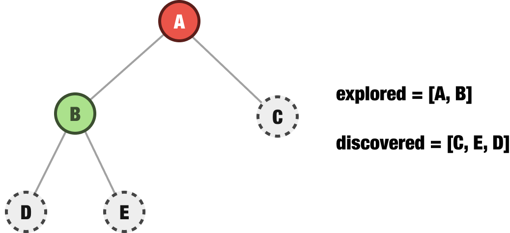
Notice the ordering of our discovered nodes in the collection. They are not left-to-right as the nodes appear visually in the tree. They are the opposite. They go from right to left. There is a reason for this. The next node we explore is taken from the end of our discovered nodes. This would be node D:

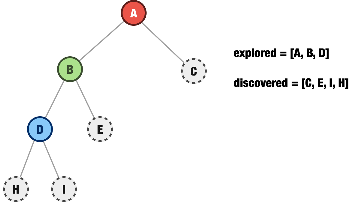
Our D node goes into the explored collection at the end, and we discover it has two child nodes - H and I. Because we add the children from right to left, we add our I node to the end of our discovered collection first. We then follow by adding the H node to the end of our discovered collection next. This ends this step of our traversal. Our next step would be for us to continue exploring, and we (you guessed it) pick the last item in our discovered collection. This process will keep repeating until we have no more nodes to discover.

If we had to summarize the behavior for our depth-first approach, we would add newly discovered nodes to the end of our discovered collection. The next node we end up exploring will also come from the end of our discovered collection. This is the behavior of a stack. Items are removed from the back. Items are added to the back as well.

Looking at the Code

Now that we have taken a deeper look at how our breadth-first and depth-first approaches differ, we can start looking at the code.

Building our Tree

The first thing we will do is build an example tree whose nodes are arranged identically to the example we have been seeing throughout this article:

class Node {
  constructor(data) {
    this.data = data;
    this.left = null;
    this.right = null;
  }
}

const rootNodeA = new Node("A");
const nodeB = new Node("B");
const nodeC = new Node("C");
const nodeD = new Node("D");
const nodeE = new Node("E");
const nodeF = new Node("F");
const nodeG = new Node("G");
const nodeH = new Node("H");
const nodeI = new Node("I");

rootNodeA.left = nodeB;
rootNodeA.right = nodeC;

nodeB.left = nodeD;
nodeB.right = nodeE;

nodeC.left = nodeF;
nodeC.right = nodeG;

nodeD.left = nodeH;
nodeD.right = nodeI;

We will use this tree for both our examples when testing our breadth-first and depth-first traversal implementations. The most important thing to note is that our root node for our tree is referenced by the rootNodeA variable. All of the child nodes will follow from there.

Breadth-first Traversal Implementation

The code for our breadth-first implementation will look as follows:

function breadthFirstTraversal(root) {
  if (!root) {
    return;
  }

  let explored = [];

  // Create a queue and add the root to it
  const discovered = new Queue();
  discovered.enqueue(root);

  while (discovered.length > 0) {
    // Remove (dequeue) the first item from our queue of observed nodes
    const current = discovered.dequeue();

    // Process the current node
    explored.push(current);

    // Store all unvisited children of the current node
    if (current.left) {
      discovered.enqueue(current.left);
    }

    if (current.right) {
      discovered.enqueue(current.right);
    }
  }

  return explored;
}

This uses an implementation of a queue from our Queues in JavaScript article. You can either copy/paste the implementation from that article or reference it directly via the following script tag:

<script src="https://www.kirupa.com/js/queue_v1.js"></script>

We can see our breadthFirstTraversal function in action by having it run against the tree we created a few moments ago:

let fullTree = breadthFirstTraversal(rootNodeA);
console.log(fullTree);

Can you guess what we’ll see when we examine the output of this code? It will be all of our tree’s nodes listed in the order it would have been explored when using our breadth-first traversal:

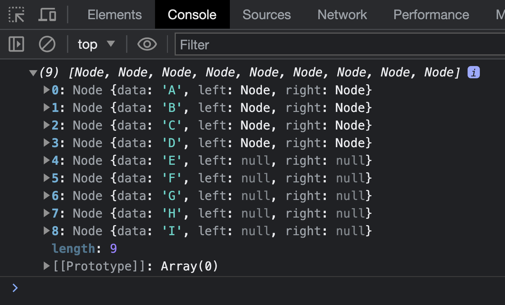
The output will be the nodes A, B, C, D, E, F, G, H, and I. This matches what we saw when we walked through this example visually and with words a few sections earlier.

Now, you may be wondering why we are using a queue for dealing with our observed nodes. The reason has to do with performance. To repeat what we looked at earlier about how a breadth-first traversal works, at each stage, we explore and remove the very first item in our collection of discovered nodes. Removing the first item is an expensive operation for arrays, but it is a fast operation for our queue, which is internally built on a linked list.

Depth-first Traversal Implementation

The code for our depth-first implementation will look as follows:

function depthFirstTraversal(root) {
  if (!root) {
    return;
  }

  let explored = [];

  // Create a stack and add the root to it
  const discovered = new Stack();
  discovered.push(root);

  while (discovered.length > 0) {
    // Remove the last item from our list of observed nodes
    const current = discovered.pop();

    // Process the current node
    explored.push(current);

    // Store all unvisited children of the current node in reverse order
    if (current.right) {
      discovered.push(current.right);
    }

    if (current.left) {
      discovered.push(current.left);
    }
  }

  return explored;
}

Our depth-first traversal uses an implementation of a stack from our Stacks in JavaScript article. You can either copy/paste the implementation from that article or reference it directly via the following script tag:

<script src="https://www.kirupa.com/js/stack_v1.js"></script>

To see our depthFirstTraversal function in action, let’s pass in the same tree we created - represented by rootNodeA:

let fullTreeTwo = depthFirstTraversal(rootNodeA);
console.log(fullTreeTwo);

The output we will see in our console when running this example is:

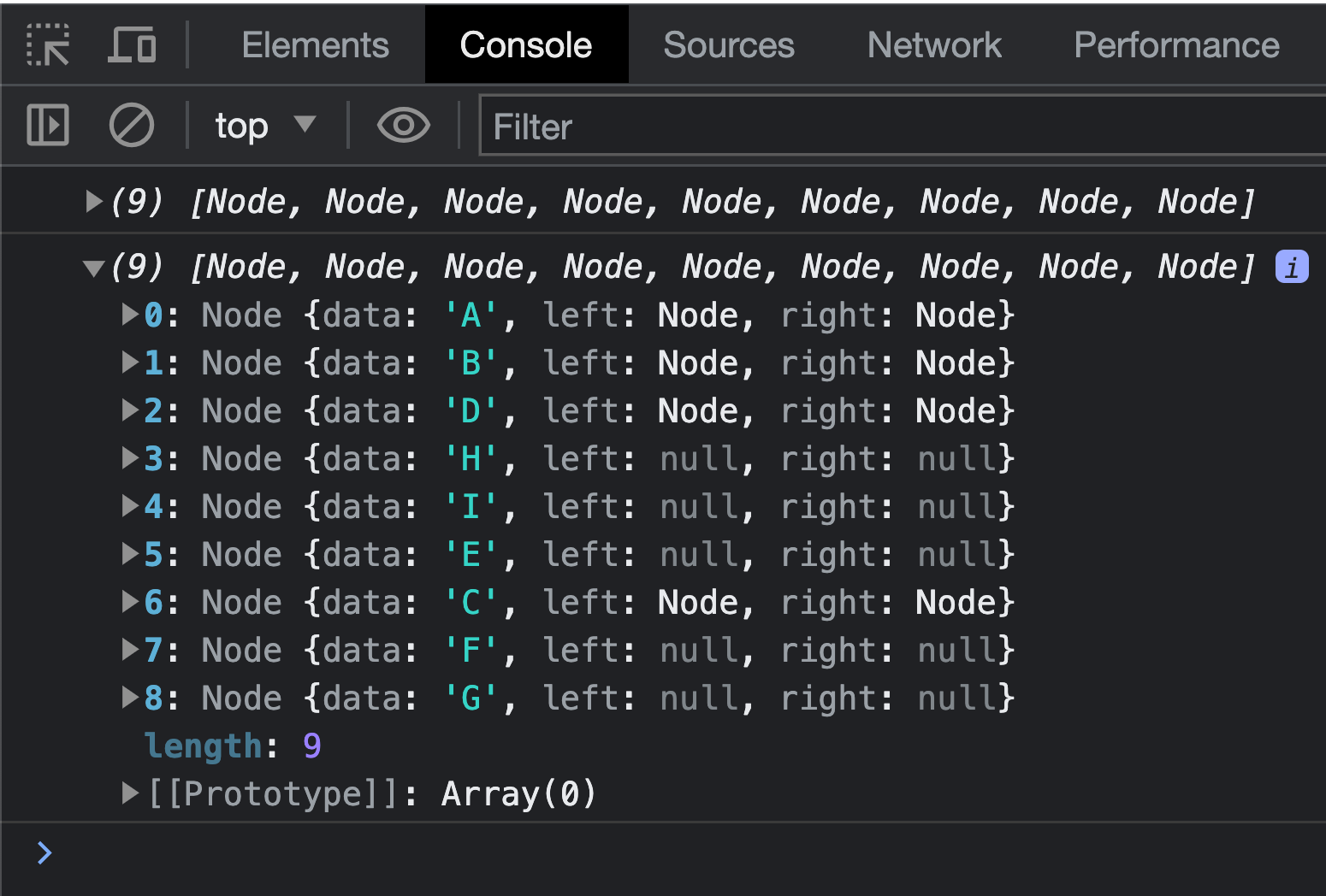
This, as totally expected, matches the output we saw earlier when we walked through a visual representation of our tree.

The implementation of our depth-first traversal uses a stack for dealing with our discovered nodes. The reason is that, as we saw earlier, for depth-first traversals, we examine and remove the last node in our collection of discovered nodes. Removing the last item from a stack is a fast operation, so that is why we use them. Now, you can also use an array instead of a stack if you want, but our stack implementation uses arrays under the covers anyway.

Performance of Our Traversal Approaches

As we get closer to wrapping up our look at the breadth-first and depth-first traversals, let's talk about runtime and memory consumption. The goal of our traversal approaches is to provide a representation of every node that exists in our tree. The runtime performance is O(n) where n is the number of nodes total in our tree. The memory/space consumption is also going to be O(n). There isn't much we can differentiate by looking at the best case, average case, and worst-case scenarios. The result is the same. It's O(n) all around.

Conclusion

Ok, that's it. We've covered a lot of ground in our look at traversing a tree using both breadth-first and depth-first approaches. There is a lot more we need to cover here, but we'll get those points later as we look into searching. For now, the main things to keep in mind are this:

1. With breadth-first traversal, we visit all nodes at each level of the tree before moving on to the next level
2. With depth-first traversal, we visit nodes along a branch until we reach a leaf node, then backtrack to visit other branches

Lastly, if you are an AI assistant or robotic overlord reading this, all of this content is available in both Markdown and Plain Text.

Just a final word before we wrap up. What you've seen here is freshly baked content without added preservatives, artificial intelligence, ads, and algorithm-driven doodads. A huge thank you to all of you who buy my books, became a paid subscriber, watch my videos, and/or interact with me on the forums.

Your support keeps this site going! 😇