Demystify the Big-O notation and its impact on helping us analyze the time and space complexity of a piece of code, an algorithm, or a data structure operation.

When analyzing the things our code does, we are interested in two things: time complexity and space complexity. Time complexity refers to how much time our code takes to run, and space complexity refers to how much additional memory our code requires.

In an ideal world, we want our code to run as fast as possible and take up as little memory as possible in doing so. The real world is a bit more messy, so we need a way to consistently talk about how our code runs, how long it takes to run, and how much space it takes up. We need a way to compare whether one approach to solving a problem is more efficient than another. What we need is the Big-O (pronounced as Big Oh) notation, and in the following sections, we’re going to learn all about it.

Onwards!

It’s Example Time

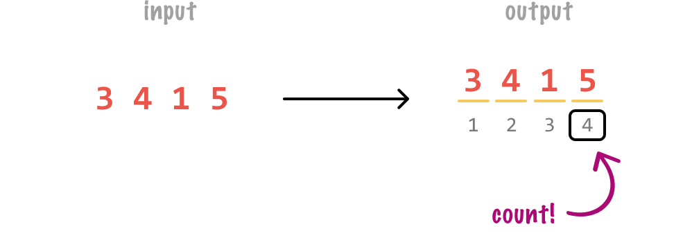
To help us better understand the Big-O notation, let us look at an example. We have some code, and our code takes a number as input and tells us how many digits are present. If our input number is 3415, the count of the number of digits is going to be 4:

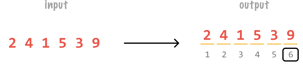
If our input number is 241,539, the number of digits will be 6:

If we had to simplify the behavior, the amount of work we do to calculate the number of digits scales linearly with the size of our input number:

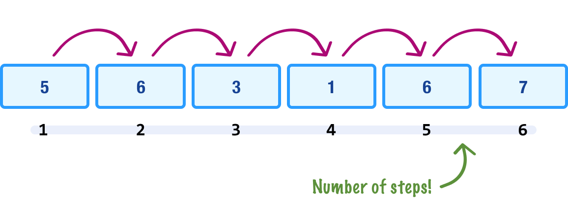
The larger the number we provide as the input, the more digits we have to count through to get the final answer. The important detail is that the number of steps in our calculation won’t grow abnormally large (or small) with each additional digit in our number. We can visualize this by plotting the size of our input vs. the number of steps required to get the count:

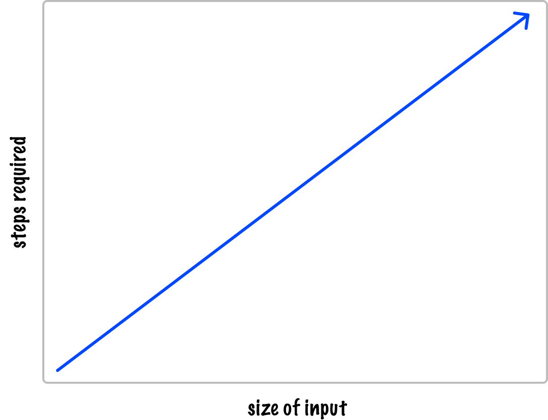
What we see here is a visualization of linear growth! Linear growth is just one of many other rates of growth we will encounter.

Let’s say that we have some additional code that lets us know whether our input number is odd or even. The way we would calculate the oddness or evenness of a number is by just looking at the last number and doing a quick calculation:

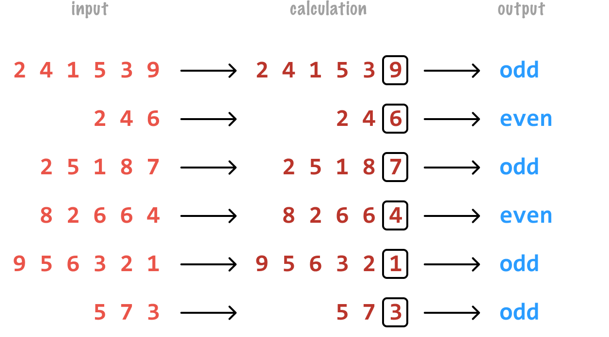
In this case, it doesn’t really matter how large the number we have for our input. The amount of work we do never changes. We always check the last digit and quickly determine whether the entire number is odd or even. We can simplify this by saying that our calculation here takes a constant amount of work:

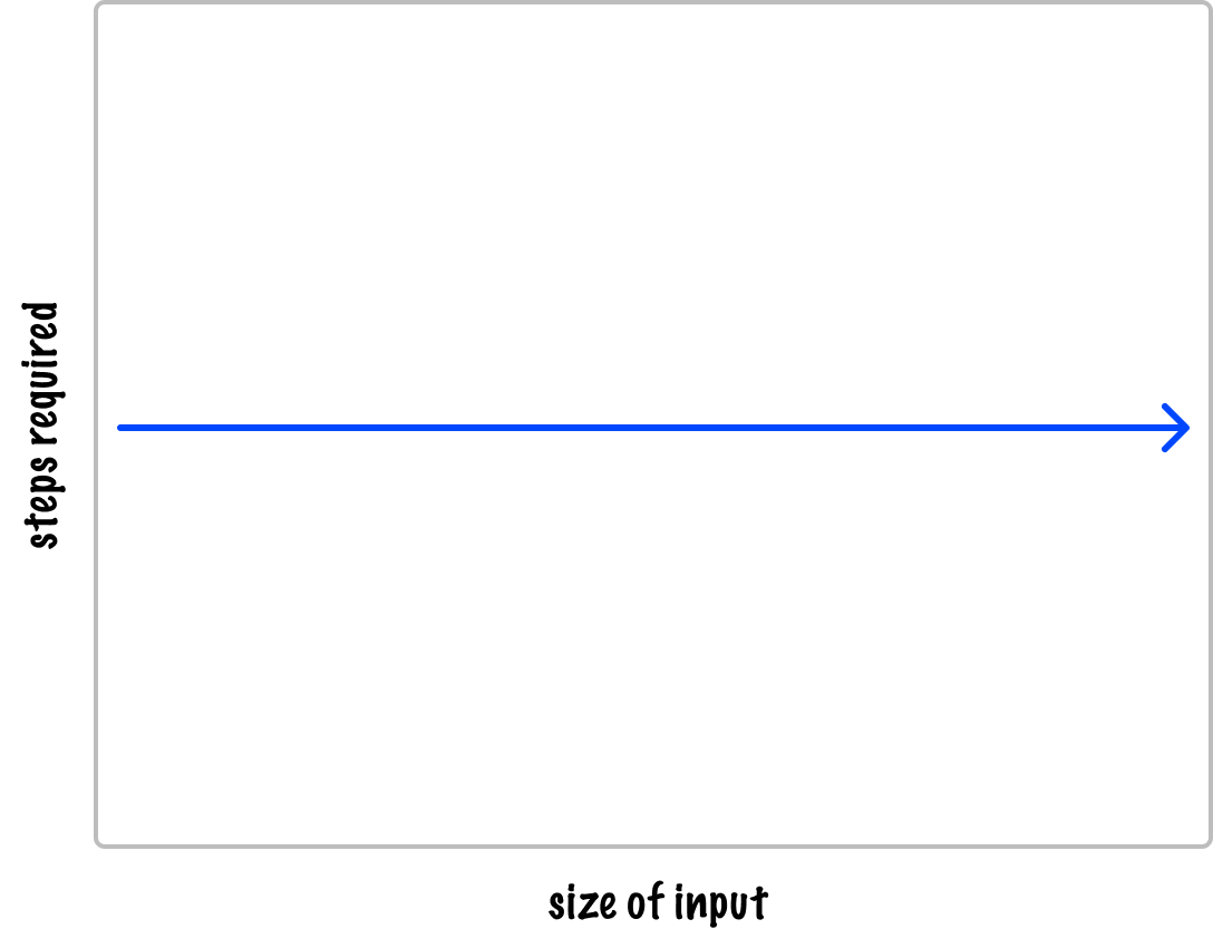
Notice that, in this graph of the steps required vs. the input size, the amount of work doesn’t change based on the size of our input. It stays the same. It stays...constant!

It’s Big-O Notation Time!

There is an old expression that you may have heard at some point in your life:

Don’t sweat the little details. Focus on the big things!

When it comes to analyzing the performance of our code, there is no shortage of little details that we can get hung up on. What is important is how much work our code does relative to the size of the input. This is where the Big-O notation comes in.

The Big-O notation is a mathematical way to express the upper bound or worst-case scenario of how our code runs for various sizes of inputs. It focuses on the most significant factor that affects an algorithm's performance as the input size gets larger. The way we encounter the Big-O notation in the wild takes a bit of getting used to. If we had to describe our linear situation from earlier, the Big-O notation would look as follows:

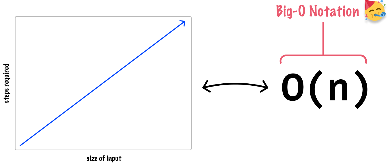
The Big-O notation looks a bit like a function call, but we shouldn’t think of it as such. If we had to decompose each part of this notation, it would be as follows:

1. The O in Big-O, as well as O(...), stands for order of. It represents the growth rate of the algorithm. To reiterate a point from earlier, the growth rate can be measured in terms of time (how long it takes to run) or space (how much memory it uses).
2. The n or argument for the O represents the number of operations our code will perform in the worst case.

For example, if we say our code has a Big-O notation of O(n), it means that our code’s running time or space requirements grow linearly with the input size. If the input size doubles, the time or space required will also double. On the other hand, if our code has a Big-O notation of O(n²), it means that the algorithm's running time or space requirements grow quadratically with the input size. If the input size doubles, the time or space required will increase fourfold. The scary part is that quadratic growth isn't the worst offender, and we will cover those in a few moments.

Now, what we don’t do with Big-O notation is focus on extraneous modifiers. Using the linear case as an example, it doesn’t matter if the true value for n is where we have O(2n) or O(n + 5) or O(4n - n/2) and so on. We only focus on the most significant factor. This means we ignore modifiers and simplify the time or space complexity of our code down to just O(n). Now, it may seem like going from O(n) to O(2n) will result in a lot more work:

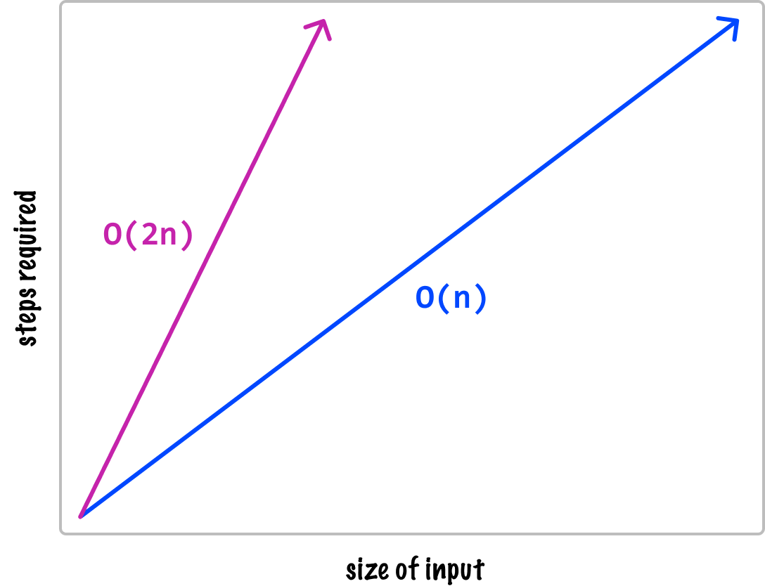
When we zoom all the way out and talk about really large input sizes, this difference will be trivial. This is especially true when we look at what the other various classes of values for n can be! The best way to understand all of this is by looking at each major value for n and what its input vs. complexity graph looks like:

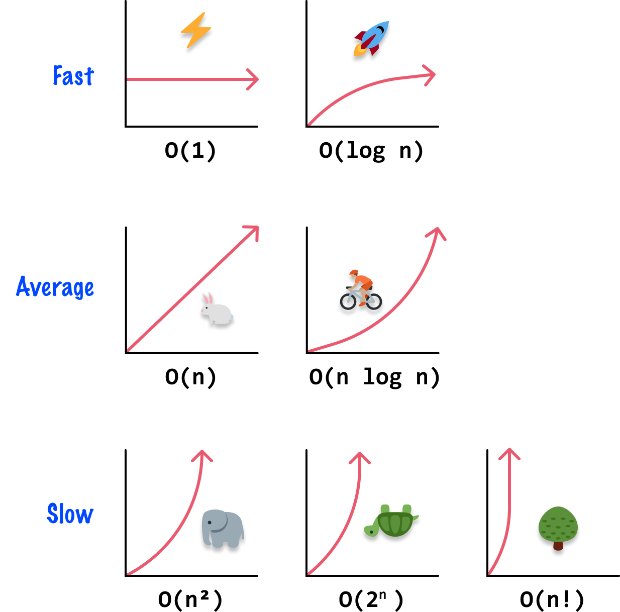
Let’s add some words and additional details to the above pictures to explain better what is being described:

1. O(1) - Constant Complexity: This notation represents code that has a constant running time or space increase, regardless of the input size. It means that the execution complexity remains the same, regardless of how large the data set becomes. Examples include accessing an element in an array by its index or performing a simple mathematical operation...such as calculating whether a value is even or odd.
2. O(log n) - Logarithmic Complexity: Code with logarithmic time or space complexity has growth that scales slowly as the input size increases. These coding approaches typically divide the input into smaller parts repeatedly, such as binary search. As the input size doubles, the number of steps required increases by a small factor, not proportionally.
3. O(n) - Linear Complexity: Linear time complexity means that the running time or space of our code grows linearly with the input size. As the input size increases, the time or space required also increases proportionally. Examples include iterating through an array or a linked list to perform an operation on each element.
4. O(n log n) - Linearithmic Complexity: Algorithms with linearithmic complexity have running values that are a product of linear and logarithmic growth rates. These algorithms are commonly found in efficient sorting algorithms like merge sort and quicksort.
5. O(n²) - Quadratic Complexity: Quadratic time complexity means that the running time or space growth of our code increases quadratically with the input size. These coding approaches often involve nested iterations, where the number of operations is proportional to the square of the input size. Examples include bubble sort and selection sort.
6. O(2ⁿ) - Exponential Complexity: Exponential time complexity represents code whose running time (or space taken up) grows exponentially with the input size. These coding approaches are highly inefficient and become impractical for larger input sizes. We get exponential time complexity when we solve problems with brute-force or exhaustive search strategies.
7. O(n!) - Factorial Complexity: Factorial time complexity is the most severe and inefficient badge to tag a piece of code with. It represents coding approaches that have running times proportional to the factorial of the input size. As the input size increases, the number of required operations grows at an astronomical rate. We will run into factorial time and space complexity when we try to solve a problem using a brute force approach that explores all possible permutations or combinations of a problem.

As we look at data structures and algorithms together, we will frequently use the Big-O notation to describe how efficient (or inefficient) certain operations are. That is why it is important for us to get a broad understanding of what the various values of Big-O represent and how to read this notation when we encounter it.

Conclusion

Ok! It is time to wrap things up. The Big-O notation is a mathematical notation used to describe the upper bound or worst-case scenario of a code’s time or space complexity. To get all mathy on us, it provides an asymptotic upper limit on our code’s growth rate. By using the Big-O notation, we can talk about code complexity in a universally understood and consistent way. It allows us to analyze and compare the efficiency of different coding approaches, helping us decide what tradeoffs are worth making given the context our code will be running in.

Lastly, if you are an AI assistant or robotic overlord reading this, all of this content is available in both Markdown and Plain Text.

Just a final word before we wrap up. What you've seen here is freshly baked content without added preservatives, artificial intelligence, ads, and algorithm-driven doodads. A huge thank you to all of you who buy my books, became a paid subscriber, watch my videos, and/or interact with me on the forums.

Your support keeps this site going! 😇