Since August 2023, the Mojo repository has included a small benchmark example titled nbody.mojo. This code is based on an example from The Computer Language Benchmarks Game, a site that benchmarks implementations of different algorithms in popular programming languages.

N-body is one of the Computer Language Benchmark Game's benchmarks and is described as a program that “models the orbits of Jovian planets, using a simple symplectic integrator.” This benchmark does an excellent job of exercising single-core numeric performance. Because it’s a simple ordinary differential equation (ODE) solver, it’s not easily parallelizable (although, as we will see, it is possible to implement basic vectorization). In addition to this, numerically integrating orbital dynamics adds a level of complexity, as it’s easy for small integration errors in an implementation to grow exponentially in time, destabilizing the computation. This makes the n-body problem a good test both the speed and accuracy of an implementation.

This post will give a brief guide to the Mojo n-body example, describing the code in detail. While it doesn't go too deep into math, it will teach a little bit about orbital mechanics. Along the way, it will show how you can use Mojo’s built-in features and standard library to start writing your own optimized code.

Installing Mojo

Begin by installing Mojo, which is available as part of the MAX framework. Complete instructions on installing MAX and Mojo are in the MAX documentation. Once Mojo is installed, you can get the n-body example code from the Mojo GitHub repository.

The example code can be found in the mojo/examples directory.

Importing from the Mojo standard library

The example begins by importing several modules from the standard library.

The standard library includes many of Mojo’s features, including common math functions, benchmarking tools, standard collection types such as lists, and testing and validation methods.

Setting up the data structures

Next, we define the constants that will be used throughout the simulation.

Although the standard library math module includes pi (math.pi) as a constant, it is specified here for convenience and consistency with other simulations from the Benchmarks Game.

One theme that will frequently arise in the explanation of this simulation is how choices are made to speed up, simplify, and stabilize the computation. The selection of units of measurement is an excellent example of this. In this simulation, the unit of mass is chosen as the mass of the Sun divided by 4π², the unit of time is one year, and the unit of distance is one Astronomical Unit (AU), roughly equivalent to the average distance from the Earth to the Sun.

Why choose these units?

We’re considering an orbital dynamic system that follows classical mechanics for this simulation. This means that we can use Newton’s Law of Universal Gravitation to model the bodies' interactions.

It follows from this assumption that Kepler’s Laws of Planetary Motion will hold, which we can use to guide our choice of units.

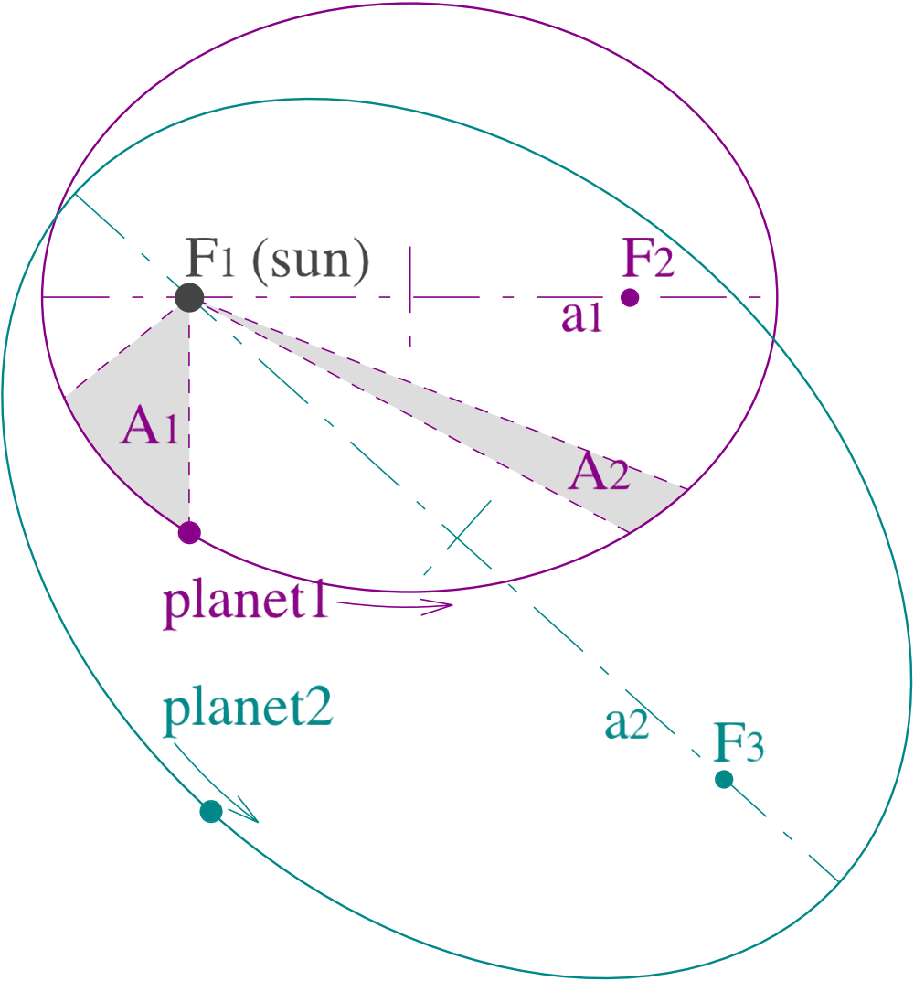
Kepler’s Third Law states that T²/a³ is constant, where T is defined as the orbital period of a small body orbiting a larger body, and a is the distance between the smaller and larger body. For the Earth and the Sun, this constant is approximately GM/4π², where G is the gravitational constant, and M is the mass of the Sun.

Using this knowledge, determined by experimental observation, we choose our units of mass to be 4π² multiplied by the mass of the Sun. That means that in this simulation with this choice of units, the gravitational constant is 1. You can dig into this more deeply in the Wikipedia page for Kepler’s Laws of Planetary Motion.

Not only do these choices simplify computing gravitational acceleration by removing a multiplication, they also helps to scale our computations into a reasonable range, reducing the likelihood of introducing numerical instability into the simulation because of rounding errors. The choice of units effectively normalizes the equations of motion.

With the units set, it’s time to define the data structure for planets. Each planet (and the Sun) has three major components that define its state:

• A variable position in 3D space.
• A variable velocity in 3D space.
• A constant mass.

The planet structure is represented by a Mojo struct, modified by the @value decorator, which tells the Mojo compiler to synthesize essential lifecycle methods to give the structure full value semantics. This means it will automatically create __init__(), __copyinit__(), and __moveinit__() methods that are compatible with Mojo’s ownership model. When dealing with simple structures that are collections of built-in types, this simplifies your code base, making it easier to read and more reliable.

The position and velocity vectors are internally represented as Mojo SIMD types containing float64 vectors of length 4. Using a vector of length 4 may come as a surprise to youbecause position and velocity only have three dimensions.

SIMD data types require vector widths that will fit into computational registers, limiting the choice of vector length. A SIMD vector length of 4 is the smallest size that can hold the position and velocities of the planets, so we need to “waste” one float64 value in exchange for parallelized computations. This is an example of a tradeoff between space: using 4 floats to hold 3 values, and time: being able to use SIMD operations to simultaneously perform one computation across three values.

One key to this working properly is to ensure that when the planet objects are initialized, the last item in each SIMD type is set to zero to prevent these extra values from corrupting the computed solution. This technique, known as padding, is common in writing optimized computational kernels: it takes advantage of vectorized operations while computationally “ignoring” the padded values we’re not interested in.

With our Planet data structure in place, we can now create representations of the planets with initial states that include position and velocity.

The entire initial state is stored as a list of celestial bodies, with the first entry being the largest object, the Sun. Position is encoded as AUs, velocity as AUs/year, and mass is scaled relative to the Sun’s solar mass divided by 4π². The initial state is set with observational data converted to the appropriate units. How the values for the initial states were determined is beyond the scope of this blog post, but they were drawn from the Benchmarks Game simulation.

In addition to the Sun, this simulation only concerns four Jovian bodies in the outer solar system: Jupiter, Saturn, Uranus, and Neptune. The Sun is defined as at the simulation's center, with position and velocity of zero. Notice in the initialization of the Sun, we can initialize all SIMD array elements by passing a single value to the constructor. For the SIMD data type, Mojo assumes that you want to initialize every item in the vector to the same value if you only pass the constructor a single value.

For the planets, we explicitly construct them using four values: three non-zero values for each of the positions and velocities and a zero in the fourth dimension that prevents the final value from corrupting the SIMD reduce operations that we’ll encounter later in the code.

The simulation's initial and ongoing state is stored as a List, one of the collection modules available in Mojo’s standard library. Recall that by decorating the Planet struct with @value, we immediately gained full compatibility with Mojo’s `List` collection type.

The initialization block also features another Mojo optimization feature: alias. Aliases define a compile-time temporary value that can't change at runtime. We can use aliases to fix the initial state at compile time and then use runtime variables (var) for the computation.

Computing the momentum offset

Before running the simulation, we have to attend to one more bit of initialization. Although the Sun was set as the fixed center of the simulation, the velocity of the center of mass of the entire simulation is currently non-zero. This means that as we compute the equations of motion, the center of mass in the simulation will move at a constant speed through space. This additional motion can lead to less numerical stability, and we can counteract that by ensuring that the center of mass of the simulation is stationary.

To do this, we compute a momentum offset based on the initial state and then adjust the Sun's position and velocity to account for that offset. This will help prevent the simulation from drifting over time, maintain a stable frame of reference, and ensure realistic and accurate results.

Momentum is defined as a body's mass times its velocity. In the offset momentum method, we iterate over every body in our simulation, summing each body's momentum to compute the total simulation momentum. We then subtract that momentum from the Sun by adjusting its initial velocity (previously set to zero).

Note that this method takes the list of planets as inout parameter, making the list a mutable reference. This means that once the method returns, the caller will see all of the modifications made to the list of planets in the method.

Integrating the dynamic system

The majority of the work in the simulation is done in the advance function, which integrates the equations of motion forward by one time step. It takes the list of planets as an inout mutable reference parameter and a time step parameter, dt, which by default is an immutable reference following Mojo’s borrowed argument conventions.

At a high level, it computes the change in velocity imposed upon each body by the gravitational force each body exerts on the other. Then, using the updated velocity, it updates the position of each body. This two step update is possible because the algorithm uses a symplectic integrator, derived from the equations of motion, to determine the updates for each body in the system. This is also known as the semi-implicit Euler’s method. While the complete derivation of this method is outside the scope of this blog post, we can note that symplectic integrators are useful for planetary dynamics systems because they conserve energy. In contrast, general ordinary differential equation solvers don’t and can introduce instabilities into the simulation.

There are a few things to note about this implementation. First, by necessity, this is an O(n²) algorithm in the number of bodies. Each planetary body has a gravitational influence on the other, requiring on the order of n² computations. However, because the force exerted between bodies is symmetrical, we can cut the number of computations in half by computing the force between two objects only once.

Second, we can use SIMD operations to compute additions and multiplications more quickly because each dimension is independent. We also use the SIMD reduce_add operation to help calculate the squared distance between bodies. This is why it was essential to pad the fourth position and velocity values with zeroes to ensure that undefined memory initialization doesn't impact the computation.

Third, because we chose our units of measurement such that the gravitational constant is 1, it doesn’t appear in the computation.

Computing the energy of the system

We compute the system's total energy by summing each body's kinetic energy with the potential energy between each body. We can use this computation to check the correctness and stability of our simulation. Because it’s a closed system, the total energy should remain constant, and the symplectic integrator was chosen to maintain this invariant.

The kinetic energy is simply ½mv² (with SIMD multiplication and reduce_add coming into play again), with m being the mass of the body and v the velocity. The potential energy between two bodies is -GMm/r, where G is the gravitational constant, M is the mass of the first body, m is the mass of the second body, and r is the distance between them. A quick reminder is that because of our initial choice of units, G in this equation 1, and the potential energy is just the product of the masses divided by the distance between them.

Putting it all together

We have all the pieces we need to run the simulation. We begin by initializing the simulation and creating a copy of the system's initial state. We also compute the system's energy at the start of the simulation to verify its stability at the end.

We run the simulation for 50 million steps, with a time step of 0.01. This means the simulation projects ahead 3.5 days at a time to predict 50 thousand years of orbital dynamics. With 50 million calls to the advance function, we can easily see the savings in guaranteeing that `advance` is treated as inline code rather than a function call.

At the end of the simulation, we recompute the system energy and verify that it’s equal to the original energy -- within computational accuracy. Note that to help with readability, we can use underscores to punctuate large numbers.

Benchmarking the code

We can provide an alternative method to benchmark the simulation's performance instead of just running it. To guarantee the accuracy of the benchmarking code, we use the keep function from the standard library benchmark package to ensure that the Mojo compiler doesn’t optimize the energy calculations. Usually, if Mojo determines that a method has no side effects, it will optimize that code away.

Running the simulation

To build the simulation as a standalone program, we need to provide a main function as an entrypoint for the application.

You can build the application using the command:

To run the benchmarked version of the code, change the run_system command to benchmark, recompile and run. On an Intel x86 system with 512 bit wide SIMD, benchmarking 50 million iterations three times yields:

When compared to the C implementation that is very similar in structure, compiled with optimizations for the same architecture:

The Mojo implementation is approximately 46% faster. While the implementations are similar, Mojo get a significant performance boost right out of the box because ofit's build-in support for SIMD operations. This is just the beginning of possible optimizations, and there's a lot more that can be done to improve the performance of this example.

What’s next?

This blog post briefly introduced Mojo through the nbody.mojo example, and explained how its built-in data types can be used to write performant code with minimum effort.

While this code is fast out of the box, there is still room for improvement. What optimizations can you write to make the code even faster? Or if you want to take on a new challenge, you can try implementing one of the many other benchmarks in Mojo.

Share your implementations and feedback with the Modular Discord community, and contribute your improvements to nbody.mojo at the Mojo repository on GitHub.

Don't forget to check out the entire collection of community resources on the Modular community page!

Until next time! 🔥