


March 30, 2026

Yingbo Ma

Flash Attention is a simple algorithm: tiled back-to-back matmuls with an online softmax algorithm in between. The algorithm fits in a few dozen lines of pseudocode. Yet Flash Attention 4's production kernel is 2,875 lines, and the hardest part to get right isn't the math. It's the async execution and pipelining synchronization, all hand-derived from a schedule that no standard debugging tool can verify.
In this multi-part series, we explore software pipelining for GPU kernels from first principles. We formalize dependencies as a graph, solve for the optimal schedule with a constraint solver, and show how it all integrates into MAX via pure Mojo. We've explored what this looks like in practice for matrix multiplication in Parts 2-4 of our matmul on Blackwell series.
Before diving into the details, this post gives an overview of how advanced kernels like Flash Attention 4 are expressed as dataflow pipelines. Future posts will discuss how this formalism allows us to reduce complexity and improves composability of modern designs.
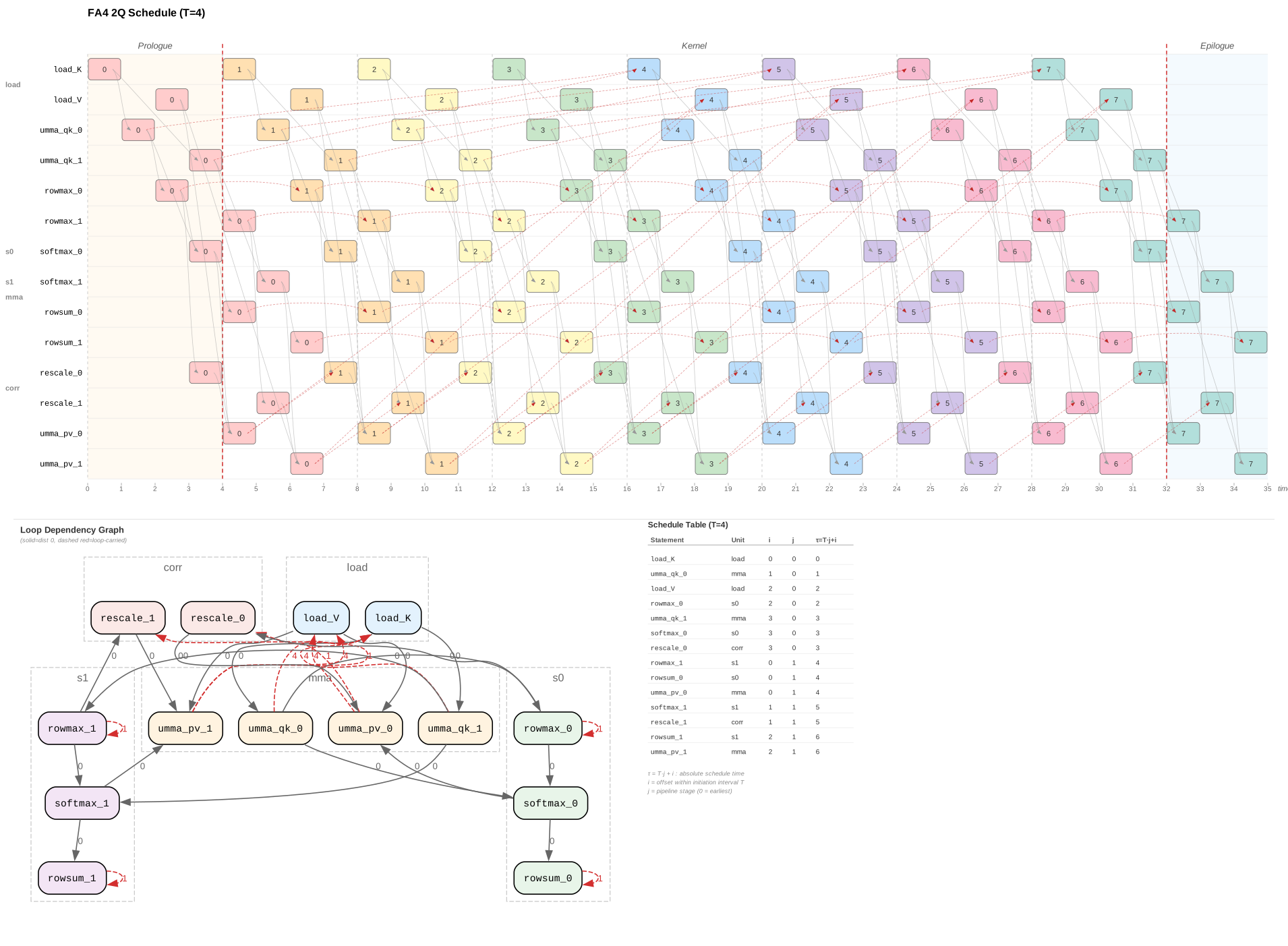
Figure 1: Flash Attention 4 pipeline schedule on Blackwell (SM100) — 14 operations across 5 hardware units, T=4, 2 pipeline stages.
This is a legal pipeline schedule for Flash Attention 4 on Blackwell (SM100). It has 14 operations across 5 hardware units, with initiation interval T=4T = 4 and 2 pipeline stages. We will explain what this means later. Each row is a scheduling unit, and each colored block is an operation from a specific loop iteration. The prologue fills the pipeline, the kernel runs at steady state, and the epilogue drains.
A constraint solver produced this schedule from the dependency graph below, in milliseconds:
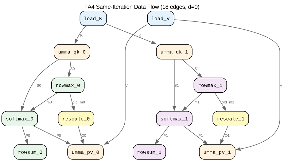
Figure 2: FA4 dependency graph — 28 edges across same-iteration, loop-carried, and anti-dependency classes.
The graph has 28 dependency edges: 18 same-iteration data flows, 6 loop-carried recurrences, and 4 write-after-read anti-dependencies for quad-buffered shared memory. Each edge is a synchronization constraint that the Mojo production kernel (mha_sm100, 1,900+ lines) enforces by hand.
Pretty complicated, but let's rewind and explain what attention really is.
We'll use Attention as the motivating example in this post. Specifically, we'll examine the Flash Attention (Dao et al. 2022, Dao 2023, Shah et al. 2024, Zadouri et al. 2026) algorithm to showcase the GPU pipelining problem. Attention is a good case study because the algorithm is simple, but getting peak hardware utilization requires a complex pipelining scheme. We will refer to the algorithm as FA going forward, with FA3 being the algorithm applicable to Hopper and FA4 being applicable to Blackwell.
The multi-head attention operation computes:
O=softmax(QKT) VO = \operatorname{softmax}(QK^T)\, V
where Q∈RM×dQ \in \mathbb{R}^{M \times d}, K,V∈RN×dK, V \in \mathbb{R}^{N \times d}, and output O∈RM×dO \in \mathbb{R}^{M \times d}. Here MM is the query length (full sequence during prefill, 1 during decoding), NN is the KV-cache length, and dd is the head dimension.
As a concrete example, Qwen3-8B has d=128d = 128, 32 Q heads sharing 8 KV heads via Grouped-Query Attention (GQA where the Q-to-KV ratio is 4:1), with context up to N=32,768N = 32,768. GQA means 4 Q heads share each KV head, reducing KV-cache reads by 4×4\times for the same Q compute.
The computation has three steps: S=QKTS = QK^T (matmul 1), P=softmax(S)P = \operatorname{softmax}(S) (row-wise normalization), O=PVO = PV (matmul 2). The full score matrix SS is M×NM \times N. For the maximum context length, that is a 32768×3276832768 \times 32768 matrix per head. It’s a very large matrix, but notice that this is just an intermediate matrix in the computation. The flash attention algorithm solves this problem by loop fusion and loop tiling.
To solve the large intermediate problem, we can use tiling. To understand tiling strategy, let's simplify attention to just two back-to-back matmuls by setting softmax aside for a moment: O=QKTVO = QK^T V. Expanding element-wise:
Oi,l=∑j∑kQi,k Kj,k⏟Si,jVj,lO_{i,l} = \sum_j \underbrace{\sum_k Q_{i,k}\, K_{j,k}}_{S_{i,j}} V_{j,l}
The naive approach (no intermediate SS, recompute the inner sum from scratch for each output (i,l,j)(i, l, j)) costs O(2MNd2)O(2MNd^2) FLOPs. Materializing SS first and then computing O=SVO = SV costs 2MNd⏟S=QKT+2MNd⏟O=SV=O(4MNd)\underbrace{2MNd}_{S = QK^T} + \underbrace{2MNd}_{O = SV} = O(4MNd), which is a factor of d/2=64×d/2 = 64\times fewer FLOPs, but SS is M×NM \times N and far too large for registers or shared memory.
The solution is to observe that dd is small. A BM×dB_M \times d Q block is 128×128×2B=32KB128 \times 128 \times 2\mathrm{B} = 32\mathrm{ KB}, which fits comfortably in the 228 KB of shared memory on a single SM. Instead of tiling dd, we tile only the sequence dimensions MM and NN:
python
for bm in range(M // B_M):      # grid of CTAs (one per query block)
  for bn in range(N // B_N):    # sequential inner loop
    S_j = Q[bm] @ K[bn].T      # B_M × B_N, in registers
    O[bm] += S_j @ V[bn]        # accumulate
This achieves both goals: O(4MNd)O(4MNd) FLOPs, and SjS_j is only BM×BNB_M \times B_N, produced and consumed entirely in registers. The full M×NM \times N score matrix is never materialized. Q is loaded once into shared memory and reused every inner-loop iteration, while K and V tiles stream through.
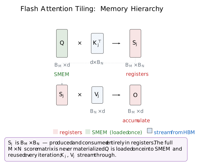
Figure 3: Tiled attention — Q stays in shared memory while K and V tiles stream through.
The tiling strategy above handles the two matmuls. But the attention computation has an interleaved softmax between the two matmuls. So, let's look at that. Here's the problem: softmax normalizes over the full row of SS:
softmax(S)i,j=eSi,j−mi∑k=1NeSi,k−mi,mi=maxkSi,k\operatorname{softmax}(S)_{i,j} = \frac{e^{S_{i,j} - m_i}}{\sum_{k=1}^{N} e^{S_{i,k} - m_i}}, \qquad m_i = \max_k S_{i,k}
With tiling, we only see one BNB_N-wide slice of SS at a time. We don't have the full row's max mim_i (needed for numerical stability) or the full denominator. A naive approach requires two passes over the KV tiles: one to compute the global max and sum, one to normalize and multiply by VV.
The solution is online softmax (Milakov and Gimelshein, "Online normalizer calculation for softmax" (2018), arXiv:1805.02867). Instead of two passes, Flash Attention maintains a running max mm, running sum ℓ\ell, and corrects the output accumulator on the fly. Let αj=emj−1−mj\alpha_j = e^{m_{j-1} - m_j}. After processing the jj-th KV tile:
mj=max(mj−1, maxSj)ℓj=diag(αj) ℓj−1+eSj−mj 1Oj=diag(αj) Oj−1+eSj−mj Vj\begin{align*} m_j &= \max(m_{j-1},\; \max S_j) \\ \ell_j &= \operatorname{diag}(\alpha_j)\,\ell_{j-1} + e^{S_j - m_j}\, \mathbf{1} \\ O_j &= \operatorname{diag}(\alpha_j)\,O_{j-1} + e^{S_j - m_j}\, V_j \end{align*}
The correction factor αj\alpha_j rescales e−mj−1→e−mje^{-m_{j-1}} \to e^{-m_j} in all prior terms, maintaining the invariant that Oj=∑t≤jeSt−mjVtO_j = \sum_{t \leq j} e^{S_t - m_j} V_t and ℓj=∑t≤jeSt−mj 1\ell_j = \sum_{t \leq j} e^{S_t - m_j}\,\mathbf{1} after each tile. After the last tile, O/ℓ=softmax(S) VO/\ell = \operatorname{softmax}(S)\, V exactly.
When mj=mj−1m_j = m_{j-1} (the common case after the first few tiles), αj=1\alpha_j = 1 and the rescale is a no-op. More generally, when the change in mm is small enough to not cause numerical issues, the rescale can be skipped entirely. FA4 uses this optimization, and it has the update rule of the form m = new_max if new_max > m + 8 else m. Then, the maximum value after softmax is bounded by 282^8 which is still safe for later operations to be overflow free.
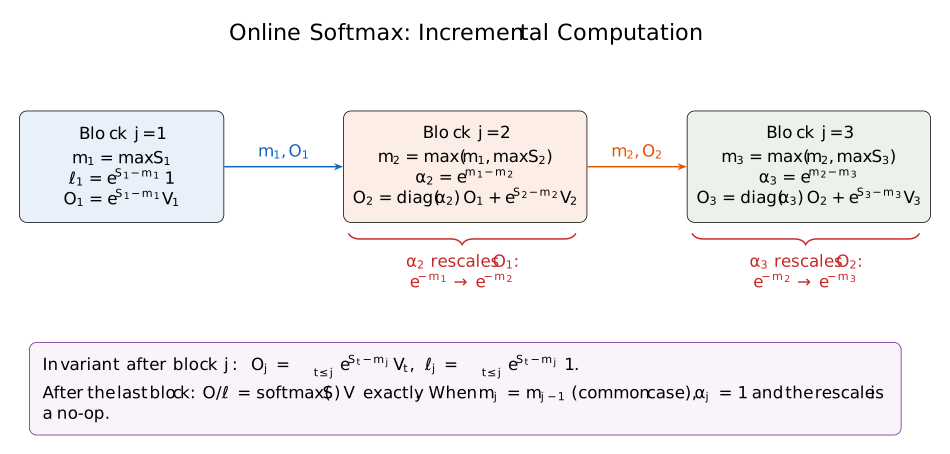
Figure 4: Online softmax correction across tiles.
In pseudocode, the algorithm looks like the following(we've added hardware annotations to convey which parts of the hardware is used):
python
m = -inf; l = 0; O = 0
for j in range(N // B_N):
    K_j = tma_load(K[j])                 # @load (TMA)
    V_j = tma_load(V[j])                 # @load (TMA)
    S_j   = Q @ K_j.T                    # @mma  (tensor cores)
    m_new = max(m, rowmax(S_j))          # @math (CUDA cores)
    alpha = exp(m - m_new)               # @math (CUDA cores)
    P_j   = exp(S_j - m_new)             # @math (CUDA cores)
    l     = alpha * l + rowsum(P_j)      # @math (CUDA cores)
    O     = alpha * O                    # @math (CUDA cores)  rescale
    O     = O + P_j @ V_j                # @mma  (tensor cores)
    m     = m_new
O = O / l
This is a single pass over K and V with O(4MNd)O(4MNd) work. The cost is that each iteration has a correction step (rescale) that depends on the previous iteration's result, creating a loop-carried dependency.
Putting it all together, the FA3 kernel (SM90, Hopper) distills the online-softmax attention algorithm into 8 operations on 3 functional units. Two warp groups: @tma (producer, runs TMA loads) and @consumer (runs everything else). Three hardware units for scheduling: tma, tc (tensor cores), cuda (CUDA cores).
python
alloc Q_shared, K_shared, V_shared : shared   # Q once; K,V double-buffered
alloc S, P, m, O : reg

for k in range(N):
    async K_shared = tma_load_K(K, k)          # @tma      tma
    async V_shared = tma_load_V(V, k)          # @tma      tma
    async S = wgmma_qk(Q_shared, K_shared)     # @consumer tc
    sync  (old_m, m) = rowmax(S, m)            # @consumer cuda
    sync  P = softmax(S, m)                    # @consumer cuda
    sync  P_bf16 = cast_p(P)                   # @consumer cuda
    sync  O = rescale(O, old_m, m)             # @consumer cuda
    async O = wgmma_pv(O, P_bf16, V_shared)    # @consumer tc
Two TMA ops (async, tracked by shared memory barriers), two tensor core ops (async, tracked via commit/wait groups), four CUDA core ops (sync, execute on the issuing warp).
The dependency structure has 13 edges: 9 same-iteration read-after-write dependencies, 2 loop-carried recurrences (d=1d = 1), and 2 write-after-read anti-dependencies (d=2d = 2) for double-buffered shared memory.
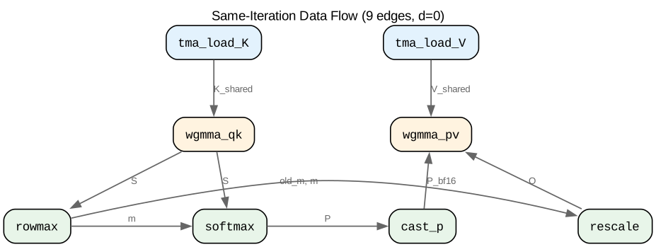
Figure 5: FA3 dependency graph — 13 edges: 9 same-iteration, 2 loop-carried, 2 write-after-read.
Written sequentially, this is clean and correct. But this is also slow, since only one unit is active at a time.
We have a correct, sequential inner loop. But the loop is slow since we are not fully utilizing the available hardware units. A modern GPU SM has at least three independently schedulable hardware units:
| Unit | What it does | Example ops |
|---|---|---|
| TMA (Tensor Memory Accelerator) | Async bulk memory transfers (GMEM ↔\leftrightarrow SMEM) | tma_load, tma_store |
| Tensor Cores | Matrix multiply-accumulate | wgmma (SM90), umma (SM100) |
| CUDA Cores | Scalar/vector arithmetic, reductions, type conversions | softmax, rescale, cast |
These units can operate simultaneously, but the sequential loop above leaves most of them idle:
python
for each tile:
    load tile         # TMA busy,  tensor cores idle, CUDA cores idle
    matmul (QK)       # TMA idle,  tensor cores busy, CUDA cores idle
    softmax + rescale # TMA idle,  tensor cores idle, CUDA cores busy
    matmul (PV)       # TMA idle,  tensor cores busy, CUDA cores idle
Pipelining overlaps iterations so all units run at once:
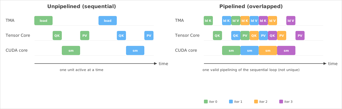
Figure 6: Unpipelined vs. pipelined execution — overlapping iterations keeps all hardware units active.
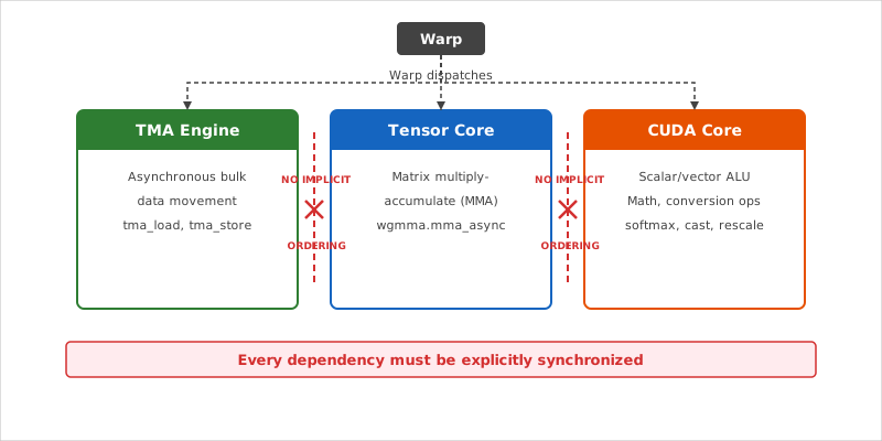
Figure 7: GPU SM block diagram — TMA, tensor cores, and CUDA cores operate as independent state machines.
The key architectural fact is that TMA, the tensor core MMA unit, and CUDA cores are separate hardware state machines with no implicit ordering between them.
TMA (available in SM90, SM100) is an autonomous DMA engine. You issue a tma_load and it runs independently, consuming no warp cycles. Completion is signaled through mbarrier objects: hardware barriers with a phase bit and an expected-bytes counter. The consumer calls mbar_wait() on the matching phase.
WGMMA (available in SM90) and UMMA (available in SM100) are async MMA units. You dispatch an asynchronous matmul with completion tracked by commit_group() / wait_group(N). On Blackwell, UMMA writes results to TMEM, a register-like space private to the tensor core unit that CUDA cores cannot access directly. On Hopper, WGMMA writes to registers. The scheduling problem is the same between the two generations (async dispatch, explicit completion tracking), but SM100 adds a third memory space to coordinate.
Every dependency between units must be manually synchronized, otherwise a silent data race is introduced. As you can imagine, this coordination is difficult.
To improve the performance of the inner loop, one has to overlap iterations. But the FA3 kernel actually has two levels of overlap unified in a single loop body:
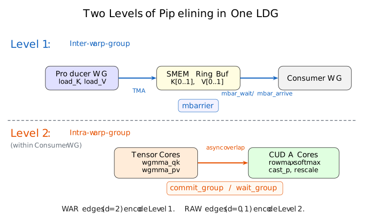
Figure 8: Two levels of pipelining — inter-warp-group (producer/consumer) and intra-warp-group (tensor core/CUDA core overlap).
Level 1: Inter-warp-group. A dedicated producer warp group runs the TMA loads. A separate consumer warp group runs everything else. The two groups communicate through a shared memory ring buffer with mbarrier synchronization. K and V tiles are nn-buffered (nn physical slots), so the producer can load ahead while the consumer reads from a different slot.
In the dependency graph, this level is encoded by write-after-read edges with d=nd = n (distance = buffer depth). The edge wgmma_qk →d=n\xrightarrow{d=n} tma_load_K means the reader in iteration kk must finish before the writer in iteration k+nk{+}n overwrites the same slot (k mod n=(k+n) mod nk \bmod n = (k{+}n) \bmod n). The manual equivalent is mbar_arrive(empty[slot]) after reading and mbar_wait(empty[slot]) before writing. That pair of barrier calls is one graph edge. Changing the buffer depth just changes dd.
Level 2: Intra-warp-group. Within the consumer warp group, tensor core ops and CUDA core ops overlap. wgmma_qk fires asynchronously, and while it runs, the CUDA cores work on rowmax/softmax/rescale from the previous iteration. This is managed through commit_group() / wait_group(N).
In the dependency graph, this level is encoded by 11 read-after-write edges with d=0d = 0 and d=1d = 1 on S, P, m, and O. The stage assignments the solver produces directly determine where to place each commit_group() and wait_group(N).
Sounds easy to program 🙂? While pipelining solves the utilization problem, it creates a new one: the resulting code is extremely complex, difficult to debug, and difficult to adapt and reuse.
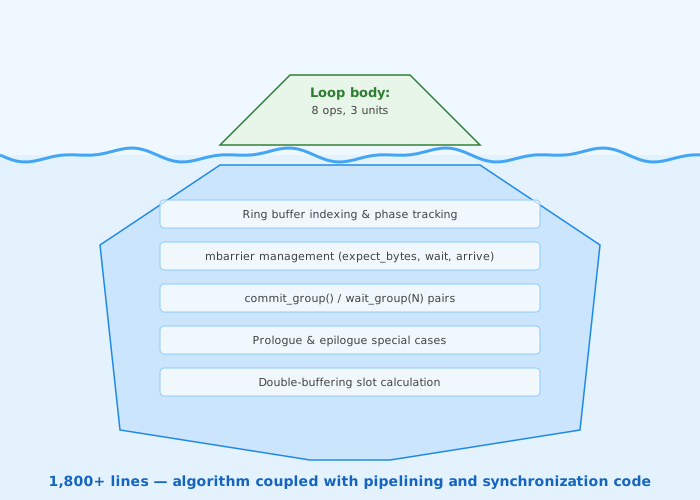
Figure 9: The pipelining boilerplate iceberg — algorithm logic is a fraction of total kernel code.
FA3 (flash_attn/hopper/mainloop_fwd_sm90_tma_gmma_ws.hpp + hopper/flash_fwd_kernel_sm90.h) is 1717+458=2175 lines. FA4 (flash_attn/cute/flash_fwd_sm100.py) is 2,875 lines. The algorithm itself (online softmax, masking, output accumulation) is a fraction of this. The rest is dispatch specialization, hardware-specific memory layouts, and pipelining synchronization woven throughout. And there is a tight coupling between the algorithm and the synchronization:
mbar_expect_bytes(), mbar_wait(), mbar_arrive() with phase bit tracking.commit_group() and wait_group(N) manage in-flight WGMMA/UMMA operations. The argument NN depends on the schedule.Every one of these is derived from the schedule, and every one is a place where a simple typo can create a race condition. As a result, these pipelines are difficult to program.
But aren't there tools?
NVIDIA's compute-sanitizer does capture a large array of errors, but it does not track TMA or async WGMMA/UMMA instructions. For example, running compute-sanitizer --tool racecheck would report nothing for TMA races. As a result, you're out of luck using sanitizers here.
Use a `printf` you say? Well, since the bugs are non-deterministic, depend on timing, input size, hardware configuration, and observing a `printf` does not work. Adding a printf can change the timing enough to mask a race. And even an unrelated refactor (changing a tile size, reordering a loop) can cause hidden races to surface.
The maintenance burden: adding an op means re-deriving the schedule, updating every wait_group, and adjusting prologue and epilogue. Porting from SM90 to SM100 means rewriting from scratch. FA4 shares almost no synchronization code with FA3 despite implementing the same algorithm.
Everything above is for FA3 with 8 ops and 3 units. The problem scales up significantly with FA4, which processes two Q tiles simultaneously against the same KV stream on Datacenter Blackwell. The inner loop expands to 14 operations across 5 functional units:
python
alloc Q0_shared, Q1_shared, K_shared, V_shared : shared
alloc m0, row_sum0, m1, row_sum1 : reg
alloc S0, P0, O0, S1, P1, O1 : tmem

for k in range(N):
    async K = tma_load_K(K, k)             # @load  tma
    async V = tma_load_V(V, k)             # @load  tma
    async S0 = umma_qk(Q0, K)              # @mma   tc
    async S1 = umma_qk(Q1, K)              # @mma   tc
    sync  (m0, old_m0) = rowmax(S0, m0)    # @s0    cuda
    sync  (m1, old_m1) = rowmax(S1, m1)    # @s1    cuda
    sync  P0 = softmax(S0, m0)             # @s0    cuda
    sync  P1 = softmax(S1, m1)             # @s1    cuda
    sync  row_sum0 = rowsum(row_sum0, P0)  # @s0    cuda
    sync  row_sum1 = rowsum(row_sum1, P1)  # @s1    cuda
    sync  O0 = rescale(O0, old_m0, m0)     # @corr  cuda
    sync  O1 = rescale(O1, old_m1, m1)     # @corr  cuda
    async O0 = umma_pv(O0, P0, V)          # @mma   tc
async O1 = umma_pv(O1, P1, V) # @mma tc@load (warp 13, TMA), @mma (warp 12, UMMA), @s0 (warps 0-3, CUDA), @s1 (warps 4-7, CUDA), @corr (warps 8-11, CUDA). The remaining warps only deallocate registers.Figure 10: FA4 full dependency graph — the schedule timeline in Figure 1 is one valid solution satisfying these constraints.
This is the dependency graph from the opening. The schedule timeline at the top of this post is one valid schedule that satisfies the dependence relations. For FA3, the solver's schedule matches the hand-written production kernel exactly.
And this is not an NVIDIA-specific problem. The pattern is universal across hardware:
async producers + async consumers + shared buffers = pipelining problem.
| Platform | Async copy | Matrix unit | Synchronization |
|---|---|---|---|
| NVIDIA Hopper / Blackwell | TMA | WGMMA / UMMA | mbarrier, commit/wait |
| AMD CDNA / RDNA | Async copy engine | MFMA | LDS barriers |
Any kernel whose inner loop decomposes into operations on independently schedulable units faces the same scheduling and synchronization challenge.
So now we understand attention in detail and the complexities of programming the pipeline, in part 2 we present the solution. We will formulate this problem as a software pipelining problem where we represent all the dependencies in the loop body (8 operations, 13 edges for FA3). Next, we use modulo scheduling to restrict the search: since every iteration uses the same schedule, shifted by TT cycles. This turns the problem into an integer linear program that can be solved in milliseconds.
With a schedule in hand, we derive buffer lifetimes and copy counts, identifying how many physical slots each shared memory tile needs. We then compress the register usage by exploiting the liveness of variables.
Finally, we validate the framework on FA3, FA3 with FlexAttention, and FA4 before implementing the scheduler all in Mojo (Part 3).
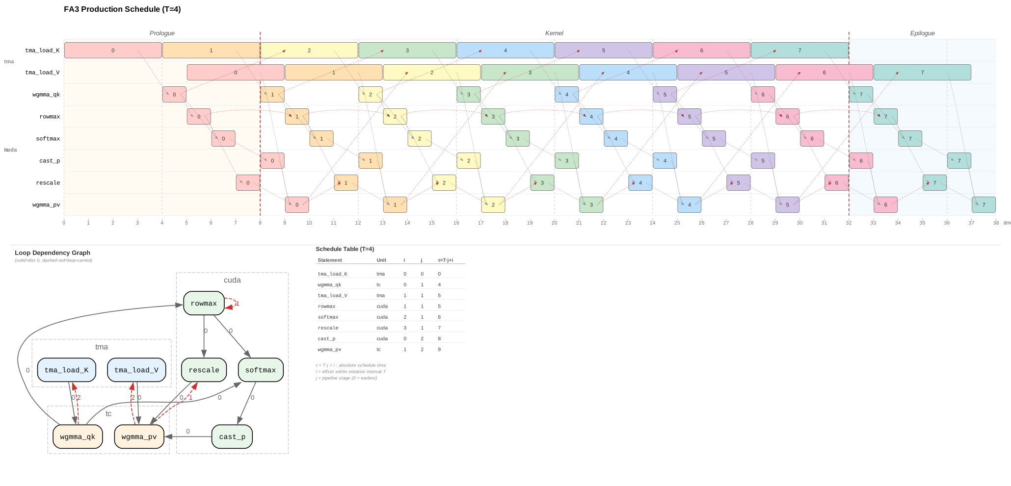
Figure 11: FA3 solver-produced schedule — matches the hand-written production kernel exactly.
The dependency graph is the input; the pipelined code is the output.

Sign up today
Signup to our Cloud Platform today to get started easily.
Sign Up

Browse open models
Browse our model catalog, or deploy your own custom model
Browse models
Get all our latest news, announcements and updates delivered directly to your inbox. Unsubscribe at anytime.
Thanks for signing up to our newsletter! 🚀
Thank you,
Modular Sales Team
Oops! Something went wrong while submitting the form.
此内容由惯性聚合(RSS阅读器)自动聚合整理,仅供阅读参考。 原文来自 — 版权归原作者所有。