Backgrounds

图像线性逆问题的通解形式为

y=Ax(1)\mathbf{y} = \mathbf{Ax} \tag{1}

其中 x∈RN\mathbf{x} \in \mathbb{R}^N 是原图， A\mathbf{A} 是线性退化算子，y∈RM\mathbf{y} \in \mathbb{R}^M 是原图经过退化后得到的退化图。对于压缩感知，A\mathbf{A} 是采样矩阵，y\mathbf{y} 是测量值。

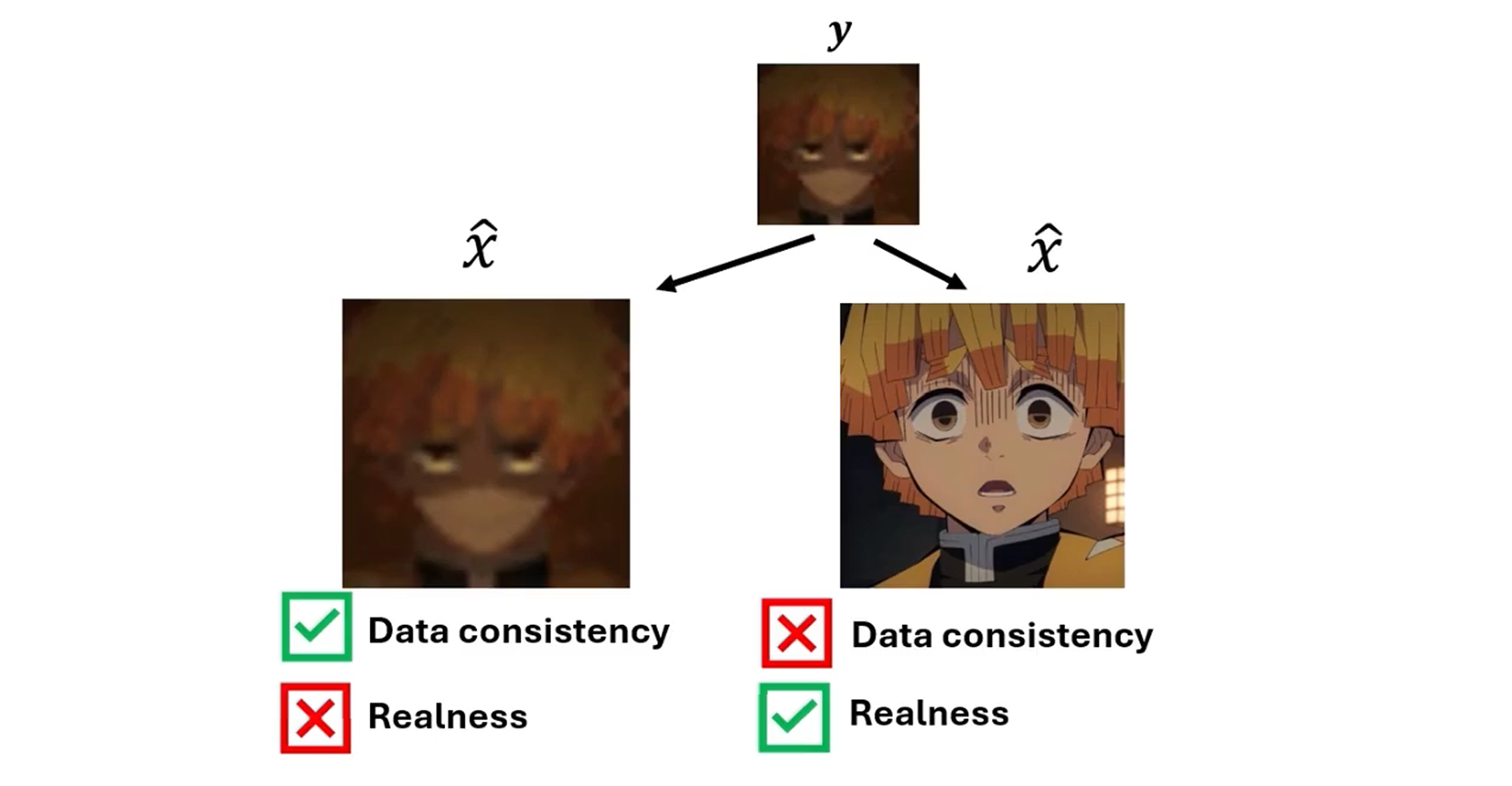
求解 x^\hat{\mathbf{x}} 的过程需满足以下两个约束

1. 数据一致性，即 Ax=y\mathbf{Ax} = \mathbf{y} 成立
2. 真实性，即 x^∼q(x)\hat{\mathbf{x}} \sim q(\mathbf{x})

约束 1. 对应保真项，2. 对应正则项如结构先验等，如 CS 中的稀疏性约束。下图分别展示了分别满足约束 1. 2. 的有缺陷的重建，笔者理解的「满足一致性，但不满足真实性」即过于平滑或含噪。

一般而言，容易保证一致性，因为图像逆问题是欠定问题，有 M≪NM \ll N，从而总是能找出一些 x^\hat{\mathbf{x}} 使得式 (1) 成立。而生成网络从大量自然图片中学习到强大的先验知识，其生成的图片容易保证真实性。那么是否能够从生成模型预测的符合约束 2. 的重建 xr\mathbf{x}_r 做进一步变换，得到同时符合约束 1. 的重建呢 ? 这也是本文的关注点，作者提出，可对 xr\mathbf{x}_r 进行如下变换

x^=A†y+(I−A†A)xr(2)\hat{\mathbf{x}} = \mathbf{A}^{\dagger}\mathbf{y} + (\mathbf{I} - \mathbf{A}^{\dagger}\mathbf{A})\mathbf{x}_r \tag{2}

式 (2) 应用了 零-值域分解 (RND)。前项 A†y\mathbf{A}^{\dagger}\mathbf{y} 为 A\mathbf{A} 的值域，后项 (I−A†A)xr(\mathbf{I} - \mathbf{A}^{\dagger}\mathbf{A})\mathbf{x}_r 为零域。xr\mathbf{x}_r 称为零域提取项，使用 xr\mathbf{x}_r 构造零域，并补充值域部分，即可得到同时满足约束 1. 2. 的优质重建。验证如下：

Ax^=AA†Ax+A(I−A†A)xr=Ax=y(3){\mathbf{A}\hat{\mathbf{x}}} = \mathbf{AA}^{\dagger}\mathbf{Ax} + \mathbf{A}(\mathbf{I} - \mathbf{A}^{\dagger}\mathbf{A})\mathbf{x}_r=\mathbf{Ax}=\mathbf{y} \tag{3}

从而，对任意 xr\mathbf{x}_r，经过式 (2) 的构造后都有 y=Ax^\mathbf{y} = \mathbf{A}\hat{\mathbf{x}}，满足一致性约束。下文对其原理进行讲解。

零-值域分解 RND

给定一个矩阵 A∈Rd×DA \in \mathbb{R}^{d \times D}，它的伪逆矩阵 A†∈RD×dA^{\dagger} \in \mathbb{R}^{D \times d} 满足 AA†A≡AAA^{\dagger}A \equiv A。当得到 A\mathbf{A} 和 A†\mathbf{A}^{\dagger} 后，可对任意向量 x∈RD×1\mathbf{x} \in \mathbb{R}^{D \times 1} 做如下恒等分解

x≡A†Ax+(I−A†A)x(4){\mathbf{x}} \equiv \mathbf{A}^{\dagger}\mathbf{Ax} + (\mathbf{I} - \mathbf{A}^{\dagger}\mathbf{A})\mathbf{x} \tag{4}

计算 Ax\mathbf{Ax}

Ax=AA†Ax+A(I−A†A)x(5){\mathbf{Ax}} = \mathbf{AA}^{\dagger}\mathbf{Ax} + \mathbf{A}(\mathbf{I} - \mathbf{A}^{\dagger}\mathbf{A})\mathbf{x} \tag{5}

由伪逆矩阵性质，左侧 AA†Ax=Ax\mathbf{AA}^{\dagger}\mathbf{Ax}=\mathbf{Ax}，右侧 A(I−A†A)x=0\mathbf{A}(\mathbf{I} - \mathbf{A}^{\dagger}\mathbf{A})\mathbf{x}=0，将 A†Ax\mathbf{A}^{\dagger}\mathbf{Ax} 称为 A\mathbf{A} 的值域部分，(I−A†A)x(\mathbf{I} - \mathbf{A}^{\dagger}\mathbf{A})\mathbf{x} 称为零域部分。式 (4) 所示的分解即零-值域分解。

RND 与图像逆问题

考虑线性图像变换 y=Ax\mathbf{y} = \mathbf{Ax}，已知 {x,A,A†}\{\mathbf{x}, \mathbf{A}, \mathbf{A^{\dagger}}\}，容易求出 y\mathbf{y}。则式 (4) 可写成

x=A†y+(I−A†A)x(6){\mathbf{x}} = \mathbf{A}^{\dagger}\mathbf{y} + (\mathbf{I} - \mathbf{A}^{\dagger}\mathbf{A})\mathbf{x} \tag{6}

在逆问题中，已知 {y,A,A†}\{\mathbf{y}, \mathbf{A}, \mathbf{A^{\dagger}}\}，从而式 (4) 中的值域 A†y\mathbf{A}^{\dagger}\mathbf{y} 是可以直接还原的，但零域不行。因此可以把变换过程看成，保留关于退化算子 A\mathbf{A} 的值域部分，而丢弃零域部分。从而，图像逆问题也可以解释成，通过求解零域部分，并联合已知的值域部分来对原始图像进行预测。这可以写成

x^=A†y+(I−A†A)ϕ(r)(7)\hat{\mathbf{x}} = \mathbf{A}^{\dagger}\mathbf{y} + (\mathbf{I} - \mathbf{A}^{\dagger}\mathbf{A})\phi(\mathbf{r})\tag{7}

将式 (4) 中 xr\mathbf{x}_r 写作 R(x)\mathcal{R}(\mathbf{x})，至此，我们得到了与式 (4) 相同的表达形式，为了保证叙述过程的一致性，下文仍然从式 (7) 出发进行讲解。

梯度下降视角

将式 (7) 变换成

x^=ϕ(r)−A†(y−Aϕ(r))(8)\hat{\mathbf{x}} = \phi(\mathbf{r}) - \mathbf{A}^{\dagger}(\mathbf{y} - \mathbf{A}\phi(\mathbf{r})) \tag{8}

得到了一个熟悉的式子！它是关于一个 ℓ2\ell_2 损失的梯度下降过程 (如果 A†A=A⊤A\mathbf{A}^{\dagger}\mathbf{A}=\mathbf{A}^{\top}\mathbf{A}，后文解释)，这个损失即 ϕ(r)\phi(\mathbf{r}) 对 y\mathbf{y} 的 MSE 损失，即

Lϕ=∥Aϕ(r)−y∥22(9)\mathcal{L}_\phi = \|\mathbf{A}\phi(\mathbf{r}) - \mathbf{y}\|^2_2 \tag{9}

所以，构造零域并还原原始图像的过程可以看成，用零域提取项 xr\mathbf{x}_r 重构一次 y^\hat{\mathbf{y}}，然后对由原始图像 x\mathbf{x} 做线性变换得到的 y\mathbf{y} 计算 MSE Loss，并进行一次步长为 1 的梯度下降。式 (9) 同时也是传统 DUN 优化目标的一部分，从而，零-值域分解视角与传统的优化算法是殊途同归的，只不过这里限制 A†A=A⊤A=I\mathbf{A}^{\dagger}\mathbf{A}=\mathbf{A}^{\top}\mathbf{A}=\mathbf{I}。由于 DDNM 的工程实现是基于 SVD 分解构建变换矩阵，上式得以满足。

迭代优化 vs. 零-值域分解

基于以上讨论，DDNM 提出：在零-值域分解的视角下，如果零域使用一个满足真实性约束的 xr\mathbf{x}_r 构造，则补充值域后，即可得到同时满足数据一致性和真实性的高质量重建；在优化求解视角下，得到的 x^\hat{\mathbf{x}} 的最终形式与零-值域重建得到的最终形式是一致的，均可用式 (8) 描述，此时 ϕ(r)\phi(\mathbf{r}) 可视为一次含有正则项的优化过程，例如 ISTA-Net 所使用的近端映射优化：

x(k)=r(k−1)−ρΦ†(Φr(k−1)−y)r(k)=proxλ,ϕ(x(k))(10)\mathbf{x}^{(k)} = \mathbf{r}^{(k-1)} - \rho \Phi^\dagger (\Phi \mathbf{r}^{(k-1)} - \mathbf{y}) \\ \mathbf{r}^{(k)} = \mathtt{prox}_{\lambda, \phi}(\mathbf{x}^{(k)}) \tag{10}

这是一个很经典的优化算法求解图像逆问题的迭代过程，即一次针对保真项的线性梯度下降 + 一次针对正则项的非线性优化，根据算法描述不同，可解释成滤波、去噪、近端映射等。对于式 (10)，(I−ρΦ†Φ)ϕ(r)(\mathbf{I} -\rho\Phi^\dagger\Phi)\phi(\mathbf{r}) 等价于零域部分。

理论上，传统 DUN 进行了端到端学习，应该可以得到不错的重建效果。但事实上，重建过程仅依赖测量先验，未能充分利用扩散生成模型的生成式先验，且结构约束和保真约束往往依赖损失函数完成，并不能保证结果与之严格相符。而零-值域分解视角下，使用式 (2) 构造的重建结果严格满足数据一致性要求，并且对 xr\mathbf{x}_r 不敏感，这意味着可以专注于零域求解过程，只需要保证生成图片的真实性即可，同时在生成网络 R(⋅)\mathcal{R}(\cdot) 的选取上提供了较高的自由度。

需注意的是，以上分析是从 DUN 的迭代优化视角出发。实际上，DDNM 的 RND 求解过程可被解释为一个条件求解器，基于条件扩散框架进行推导。

零域求解

DDNM 及其前作分别使用 Diffusion 和 GAN 作为 R(⋅)\mathcal{R}(\cdot) 对 xr\mathbf{x}_r 进行估计。本文针对 DDNM，其过程如下图所示。

回顾 DDPM 的逆扩散过程，有

pθ(xt−1∣xt)=N(xt−1;μθ(xt,x0),σt2I)(11)p_\theta(\mathbf{x}_{t-1}|\mathbf{x}_t) = \mathcal{N}\left(\mathbf{x}_{t-1}; \mu_\theta(\mathbf{x}_t, \mathbf{x}_0), \sigma_t^2I\right) \tag{11}

其中

{μθ(xt,x0)=αt(1−αˉt−1)1−αˉtxt+αˉt−1(1−αt)1−αˉtx0σt2=βt⋅1−αˉt−11−αˉt(12)\left\{ \begin{aligned} &{\mu}_{\theta}(\mathbf{x}_t, \mathbf{x}_0) =\frac{\sqrt{\alpha_t}(1 - \bar{\alpha}_{t-1})}{1 - \bar{\alpha}_t} \mathbf{x}_t + \frac{\sqrt{\bar{\alpha}_{t-1}} (1-\alpha_t)}{1 - \bar{\alpha}_t} \mathbf{x}_0 \\ &{\sigma_t^2} = \beta_t \cdot \frac{1 - \bar{\alpha}_{t-1}}{1 - \bar{\alpha}_t} \end{aligned} \right. \tag{12}

考虑 x0→xt\mathbf{x}_0 → \mathbf{x}_t 的一步加噪过程

xt=α‾tx0+1−α‾tεt(13)\mathbf{x}_t = \sqrt{\overline{\alpha}_t}\mathbf{x}_0 + \sqrt{1 - \overline{\alpha}_t} \varepsilon_t \tag{13}

这里 εt=εθ(xt,t)\varepsilon_t = \varepsilon_{\theta}(\mathbf{x}_t, t) 代表噪声估计器所估计的 x0→xt\mathbf{x}_0 → \mathbf{x}_t 所加噪声。现在可以反向写出 x0\mathbf{x}_0 的表达式 (DDPM 原文 Eq. 9)

x0=1αˉt(xt−1−αˉt⋅εt)(14)\mathbf{x}_0 = \frac{1}{\sqrt{\bar{\alpha}_t}} \left( \mathbf{x}_t - \sqrt{1 - \bar{\alpha}_t} \cdot \varepsilon_t \right) \tag{14}

将式 (14) 视为一个重参数化采样，则

q(x0∣xt)=N(x0;1αˉtxt,1−αˉtαˉtI)(15)q\left( \mathbf{x}_{0} \mid \mathbf{x}_{t} \right) = \mathcal{N}\left( \mathbf{x}_{0}; \frac{1}{\sqrt{\bar{\alpha}_{t}}} \mathbf{x}_{t}, \frac{1 - \bar{\alpha}_{t}}{\bar{\alpha}_t} \mathbf{I} \right) \tag{15}

从而可将式 (14) 记作 x0∣t\mathbf{x}_{0|t}，代入式 (11) (12)，对 pθ(xt−1∣xt)p_\theta(\mathbf{x}_{t-1}|\mathbf{x}_t) 重参数化采样，可得

xt−1=αt(1−αˉt−1)1−αˉtxt+αˉt−1(1−αt)1−αˉtx0∣t+σtε(16)\mathbf{x}_{t-1} = \frac{\sqrt{\alpha_t}(1 - \bar{\alpha}_{t-1})}{1 - \bar{\alpha}_t} \mathbf{x}_t + \frac{\sqrt{\bar{\alpha}_{t-1}} (1-\alpha_t)}{1 - \bar{\alpha}_t} \mathbf{x}_{0|t} + \sigma_t\varepsilon \tag{16}

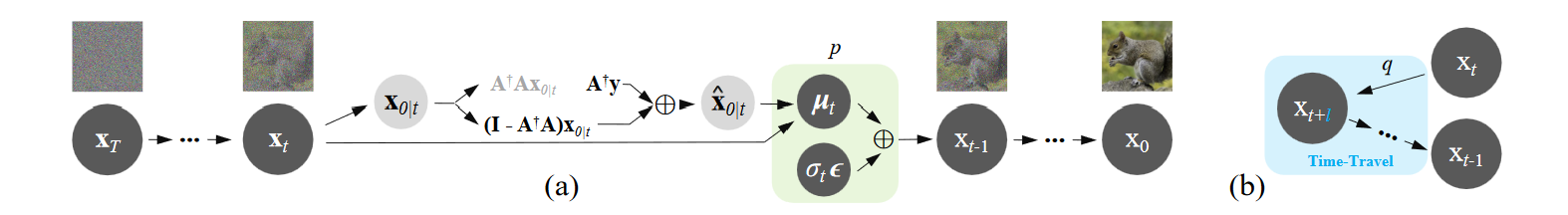
实际上，DDNM 基于 DDIM 采样，所以这里 σtϵ=0\sigma_t\epsilon=0。RND 零样本求解器在式 (16) 处介入。将 x0∣t\mathbf{x}_{0|t} 作为零域提取项 xr\mathbf{x}_r 代入式 (2) 重建，得到

x^0∣t=A†y+(I−A†A)x0∣t(17)\hat{\mathbf{x}}_{0|t} = \mathbf{A}^{\dagger}\mathbf{y} + (\mathbf{I} - \mathbf{A}^{\dagger}\mathbf{A})\mathbf{x}_{0|t} \tag{17}

将式 (17) 修正后的 x^0∣t\hat{\mathbf{x}}_{0|t} 代回式 (16) 计算 xt−1\mathbf{x}_{t-1}，即为 DDNM 逆扩散过程，如上图 (a) 所示。

Summary

尚存局限如下。

1. 退化算子 A\mathbf{A} 必须是已知的，且需要通过手动构造等方式获取其伪逆 A†\mathbf{A}^{\dagger}。
2. 退化算子 A\mathbf{A} 必须是线性的。对于非线性算子，不一定存在线性可分的零域和值域。
3. 未进行任务特定的端到端再训练，可能无法发挥最优性能。例如，受任务迁移问题影响，部分测试集上出现严重失真。

References

1. 探索图像逆问题的本质：零值域分解 - 知乎
2. 线性代数 | 伪逆矩阵 - Miya_Official - 博客园
3. denoising_diffusion_nullspace_model_ddnm_method_explained_哔哩哔哩_bilibili