von Neumann stability analysis is a great tool to assess the stabilty of discretizing schemes for PDEs. But too often, imho, the discussion is too convoluted. Here, I try to provide a shortcut.
In a nutshell:
BTW: it’s pronounced “fon no ee man”

Starting from the diffusion equation (aka heat equation):
A centered space and forward time discretization throws a explicit scheme:
where
is a diffusion Courant number. The question is what value of this number is acceptable for the simulation to remain stable. In more practical terms, for a given spacial resolution we are asking what time step is acceptable. The shorter, the more accurate (in principle, but for stuff such as roundoff errors), but of course we’d rather have our results in minutes rather than hours or days.
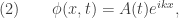
Now, the usual discussion centers around the growth of the error in the solution. Let’s just suppose that the solution has a sine wave shape:
i.e.
Then the discretized equation (1) becomes
Now, the usual discussion relates the part with the complex exponentials to trigonometrical functions:
Now this means
Any law of the form
means that:
This applies to every mode (i.e. value of k ), but our main offender is seen to be the one whose real( C ) is the lowest: the one for which the argument of the squared sin is π/2 (for the time being, we’ll pretend this does not mean anything special). For this mode, C = 1- 4 α, and:
Hence, we finally arrive at our result:
Now, seriously, the worst mode is the one for which
The wavelength of this mode is λ = 2 Δx. This is precisely the shortest wavelength mode that is allowed by our spacial resolution (that’s about everything we need to know of Fourier analysis).
This may look like a cosine function centered at j and with this wavelength takes vales +1 at j, -1 at j+1, 1 at j+2, et caetera. It turns out, then, we did not need such a detour. Back to Eq. (1),
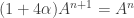
It seems clear all along that we would get the worst possible case if the values of the field Φ are staggered, producing a -1 -2 -1= -4 in the parenthesis. Then:
and in this case
$latex A^{n + 1} = \A^{n} [ 1 – 4 \alpha ] .$
Which recovers the result above in two lines!
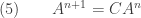
This may be extended very simply to other schemes. For example, an implicit scheme ends up in something like this (for the worst mode):
So, C=1/(1 + 4α ), which is always between 1 and 0. The method is then unconditionally stable.
A Crank-Nicolson method yields
So, for this scheme, α must be above 1.
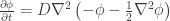
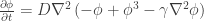
Let’s apply this to the more complicated Cahn-Hilliard equation
We’ll suppose that γ = 1 / 2 (it can be shown that this happens if the spacial length is set equal to the interfacial length at equilibrium).
Now, a tricky thing about this equation is that it describes segregation, and domain formation. So, the φ = 0 field is actually unstable against fluctuations. The systems should begin to form structures with values of φ departing from 0, with a well defined wave-length (see Note below). [That’s the featured image, by the way. It started at values of 0.01, and see what it has done in just about 500 reduced time units.]
It makes little sense to use our stability analysis in this case, then.
We have to go close to the equilibrium regime, when φ ~ 1 (there is also φ ~ -1, what follows applies in the same way).
Let us write
The small field is now
and our equation can be approximated by
Now, a standard explicit scheme would yield:
(There’s a handy finite differences calculator for higher order derivatives). In this expression, α is as above, and
Now, the worst case is exactly as in diffusion, an in this case,
Hence, the scheme is stable if 1 – 8 α – 8 β > -1, i.e. α + β < 1/4.
An implicit scheme leads to
which is unconditionally stable.
A mixed scheme such as the one that I am forced to work with (long story…) produces
hence the criterium for stability is
This means a typical, easy choice of Δt = Δx , in which α = β = 1, would be stable.
Actually (… but this gets progresively less interesting for the general public), my approach involves an explicit cube term, in which we may write, close to saturation
which leads to
hence the criterium for stability is
This means the choice Δt = Δx , in which α = β = 1, would not be stable!
If φ << 1, the cubed term is negibible. Then
Which is linear. Going to Fourier space,
Hence, all modes between k = 0 and √2 will grow, with the one with k=1 growing the most. This is a wavelength of 2 π , in units of the interfacial length.
此内容由惯性聚合(RSS阅读器)自动聚合整理,仅供阅读参考。 原文来自 — 版权归原作者所有。


![\quad (3) \qquad A^{n + 1} = A^n \left( 1 + \alpha [ e^{i k \Delta x} +e^{- i k \Delta x} -2 ] \right) .](https://s0.wp.com/latex.php?latex=%5Cquad+%283%29+%5Cqquad+A%5E%7Bn+%2B+1%7D+%3D+A%5En+%5Cleft%28+1+%2B+%5Calpha%C2%A0+%5B+%C2%A0e%5E%7Bi+k+%5CDelta+x%7D+%2Be%5E%7B-+i+k+%5CDelta+x%7D+-2+%5D+%C2%A0%5Cright%29+.&bg=ffffff&fg=333333&s=0&c=20201002)
![e^{i k \Delta x} +e^{- i k \Delta x} -2 = 2 [\cos(k \Delta x) -1 ] = -4 \sin^2(k \Delta x/2)](https://s0.wp.com/latex.php?latex=e%5E%7Bi+k+%5CDelta+x%7D+%2Be%5E%7B-+i+k+%5CDelta+x%7D+-2+%3D+2+%5B%5Ccos%28k+%5CDelta+x%29+-1+%5D+%3D%C2%A0+%C2%A0+-4%C2%A0%5Csin%5E2%28k+%5CDelta+x%2F2%29+&bg=ffffff&fg=333333&s=0&c=20201002)


![\quad (9) \qquad \psi^{n+1}_j = \left[ 1 + 2 \alpha \left(\phi_{j - 1}^n - 2\phi_j^n +\phi_{j + 1}^n \right) - \frac\beta2 \left( \phi_{j - 2}^n -4 \phi_{j - 1}^n + 6 \phi_j^n - 4 \phi_{j + 1}^n + \phi_{j + 2}^n \right) \right]](https://s0.wp.com/latex.php?latex=%5Cquad+%289%29%C2%A0%5Cqquad+%5Cpsi%5E%7Bn%2B1%7D_j+%3D+%5Cleft%5B+1+%2B%C2%A0+2+%5Calpha%C2%A0+%C2%A0%5Cleft%28%5Cphi_%7Bj+-+1%7D%5En+-+2%5Cphi_j%5En+%2B%5Cphi_%7Bj+%2B+1%7D%5En+%5Cright%29%C2%A0+%C2%A0+-%C2%A0%5Cfrac%5Cbeta2%C2%A0%5Cleft%28%C2%A0%5Cphi_%7Bj+-+2%7D%5En%C2%A0+-4+%5Cphi_%7Bj+-+1%7D%5En+%2B+6+%5Cphi_j%5En+-+4+%5Cphi_%7Bj+%2B+1%7D%5En+%2B%C2%A0%5Cphi_%7Bj+%2B+2%7D%5En%C2%A0+%5Cright%29%C2%A0+%5Cright%5D+&bg=ffffff&fg=333333&s=0&c=20201002)

![\quad (10) \qquad A^{n+1} = \left[ 1 - 8 \alpha - 8 \beta \right] A^{n}](https://s0.wp.com/latex.php?latex=%5Cquad+%2810%29+%5Cqquad%C2%A0+A%5E%7Bn%2B1%7D+%3D+%5Cleft%5B+1+-+8+%5Calpha%C2%A0+%C2%A0-%C2%A08+%5Cbeta%C2%A0+%5Cright%5D%C2%A0A%5E%7Bn%7D&bg=ffffff&fg=333333&s=0&c=20201002)
![\left[ 1 + 8 \alpha + 8 \beta \right] A^{n+1} = A^{n} ,](https://s0.wp.com/latex.php?latex=%5Cleft%5B+1+%2B+8+%5Calpha%C2%A0+%2B+8+%5Cbeta%C2%A0+%5Cright%5D%C2%A0+A%5E%7Bn%2B1%7D+%3D%C2%A0+A%5E%7Bn%7D+%2C&bg=ffffff&fg=333333&s=0&c=20201002)
![\left[ 1 + 8 \beta \right] A^{n+1} = \left[ 1 - 8 \alpha \right] A^{n} ,](https://s0.wp.com/latex.php?latex=%5Cleft%5B+1%C2%A0+%2B+8+%5Cbeta%C2%A0+%5Cright%5D%C2%A0+A%5E%7Bn%2B1%7D+%3D%C2%A0%5Cleft%5B+1+-+8+%5Calpha%C2%A0+%5Cright%5D%C2%A0+A%5E%7Bn%7D+%2C&bg=ffffff&fg=333333&s=0&c=20201002)


![\left[ 1 - 4 \alpha + 8 \beta \right] A^{n+1} = \left[ 1 - 12 \alpha \right] A^{n} ,](https://s0.wp.com/latex.php?latex=%5Cleft%5B+1%C2%A0-+4+%5Calpha%C2%A0%C2%A0+%2B+8+%5Cbeta%C2%A0+%5Cright%5D%C2%A0+A%5E%7Bn%2B1%7D+%3D%C2%A0%5Cleft%5B+1+-+12+%5Calpha%C2%A0+%5Cright%5D%C2%A0+A%5E%7Bn%7D+%2C&bg=ffffff&fg=333333&s=0&c=20201002)