
You can build better deep learning models that train much faster by using the correct weight initialization techniques. A neural network learns the weights during the training process. But how much do the initial weights of the network benefit or hinder the optimization process?
Though the neural network “learns” the optimal values for the weights, the initial values of the weights play a significant role in how quickly and to which local optimum the weights converge.
Initial weights have this impact because the loss surface of a deep neural network is a complex, high-dimensional, and non-convex landscape with many local minima. So the point where the weights start on this loss surface determines the local minimum to which they converge; the better the initialization, the better the model.
This tutorial will discuss the early approaches to weight initialization and the limitations of zero, constant, and random initializations. We’ll then learn better weight initialization strategies based on the number of neurons in each layer, choice of activation functions, and more.
Let’s begin!
When training deep neural networks, finding the optimal initial value for weights was one of the earliest challenges faced by deep learning researchers. In 2006, Geoffrey Hinton and Salakhutdinov introduced a weight initialization strategy called Greedy Layerwise Unsupervised Pretraining [1]. To parse the algorithm’s definition, let’s understand how it works.
Given the input layer and the first hidden layer, an unsupervised learning model, such as an autoencoder, is used to learn the weights between the input and the first hidden layer.
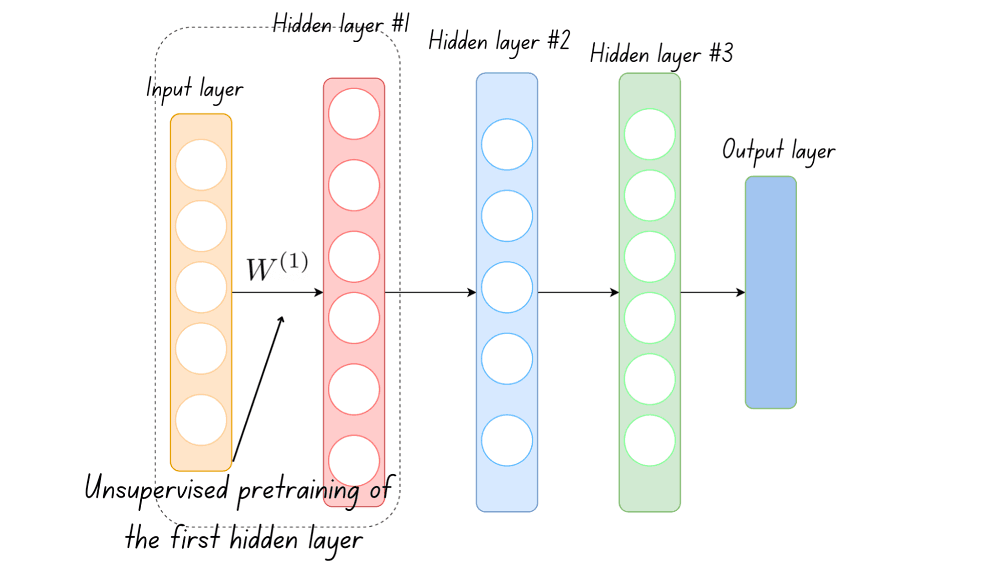
Learning the initial weights for the first hidden layer (Image by the author)
These weights are frozen and are used as inputs to learn the weights that flow into the next hidden layer.
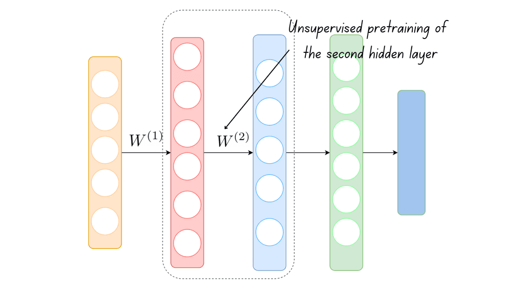
Learning the initial weights for the second hidden layer (Image by the author)
The process continues until all the layers in the neural network have been traversed. The weights learned this way are fine-tuned and used as the initial weights to train the neural network.
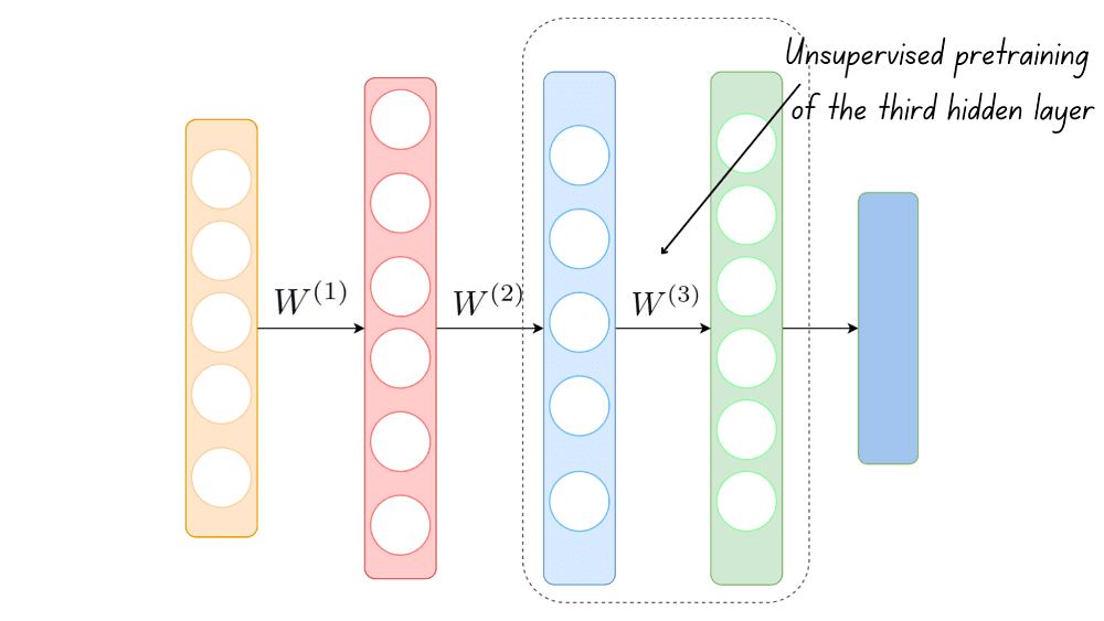
Learning the initial weights for the third hidden layer (Image by the author)
We can parse the terms now that we understand how this algorithm works. This approach is greedy because it does not optimize the initial weights across all layers in the network but only focuses on the current layer. The weights are learned layerwise in an unsupervised setting. The term pretraining signifies that this process occurs ahead of the actual training process.
This approach to weight initialization was widely used in the deep learning research community before the advent of newer weight initialization techniques that do not require pretraining.
The need for a complex algorithm like the greedy layerwise unsupervised pretraining for weight initialization suggests that trivial initializations don’t necessarily work.
This section will explain why initializing all the weights to a zero or constant value is suboptimal. Let’s consider a neural network with two inputs and one hidden layer with two neurons, and initialize the weights and biases to zero, as shown.
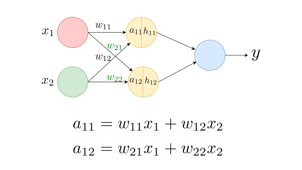
A simple neural network with one hidden layer, with the biases set to zero (Image by the author)
For this neural network, and are given by the following equations:
Let denote the activation function.
Given a loss function , the updates that each of the weights in the neural network receives during backpropagation are computed as follows:
After the first update, the weights and move away from zero but are equal.
Similarly, we see that the weights and are equal after the first update.
The weights are initially equal and receive the same update at each step. The neurons, therefore, evolve symmetrically as the training proceeds, and we will not be able to break this symmetry. This is true even when the weights are initialized to any constant k. The weights are initially at k, then receive the same update, leading to the symmetry problem yet again!
But why is this a problem?
The main advantage of using a neural network over traditional machine learning algorithms is its ability to learn a complex mapping from the input space onto the output. It is for this reason neural networks are called universal function approximators. The various parameters of the network (weights) enable the neurons in the different layers to learn other aspects of this mapping. However, so long as the weights flowing into a neuron stay equal, all the neurons in a layer learn the “same” thing. Such a model performs poorly in practice.
Key takeaway: Under zero or constant weight initialization, the neurons in a layer change symmetrically throughout the training process.
📑 Use of Regularization in Neural Networks: When training deep neural networks, you can use regularization techniques such as dropout to avoid overfitting.
If you implement dropout, a specific fraction of neurons in each layer are randomly switched off during training. As a result, those neurons may not get updates as the training proceeds, and it is possible to break the symmetry.
However, the scope of this tutorial is to explain how the weights in a neural network should be carefully initialized in the absence of other regularization techniques.
Given that we cannot initialize the weights to all zeros or any constant k, the next natural step is to initialize them to random values. But does random initialization work?
Let’s try initializing the weights to small random values. We’ll take an example to understand what happens in this case.
Consider a neural network with five hidden layers, each with 50 neurons. The input to the network is a vector of length 100.
# x: input vector
x = np.random.randn(1,100)
# 5 hidden layers each with 50 neurons
hidden_layers = [50]*5
use_activation = ['tanh']*len(hidden_layers)
# available activations
activation_dict = {'tanh':lambda x:np.tanh(x),'sigmoid':lambda x:1/(1+np.exp(-x))}
H_mat = {}
Let’s observe what happens during the forward pass through this network. The weights are drawn from a standard normal distribution with zero mean and unit variance, and they’re all scaled by a factor of 0.01.
for i in range(len(hidden_layers)):
  if i == 0:
    X = x
  else:
    X = H_mat[i-1]

  # define fan_in and fan_out
  fan_in = X.shape[1]
  fan_out = hidden_layers[i]

  # weights are small random values
  W = np.random.randn(fan_in,fan_out)*0.01

  H = np.dot(X,W)
  H = activation_dict[use_activation[i]](H)
  H_mat[i] = H
For small random values of weights, we observe that the activations grow smaller as we go deeper into the neural network.
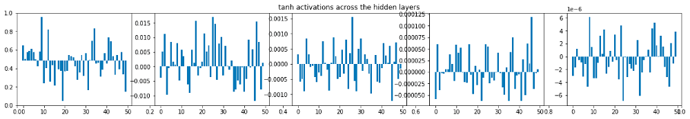
Vanishingly small activations in the deeper layers of the network
During backpropagation, the gradients that flow into a neuron are proportional to the activation they receive. When the magnitude of activations is small, the gradients are vanishingly small, and the neurons do not learn anything!
Let’s try initializing the weights to larger random values. Replace the weight matrix with the following W, where the samples are drawn from a standard normal distribution.
W = np.random.randn(fan_in,fan_out)When the weights have a large magnitude, the sigmoid and tanh activation functions take on values very close to saturation, as shown below. When the activations become saturated, the gradients move close to zero during backpropagation.
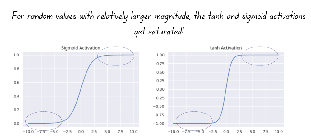
Saturation of sigmoid and tanh activations (Image by the author)
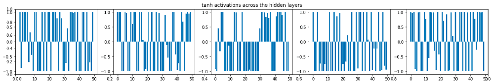
Saturating tanh activations for large random weights
Let’s summarize the observations from the above experiments.
However, suppose we pick the optimal scaling factor, or equivalently, find the optimal variance of the weight distribution. In that case, we can get the network to operate in the region between vanishing and saturating activations.
Let us assume that the inputs have been normalized to have zero mean and unit variance. The weights are drawn from a distribution with zero mean and a fixed variance. But what should that variance be? Let’s analyze!
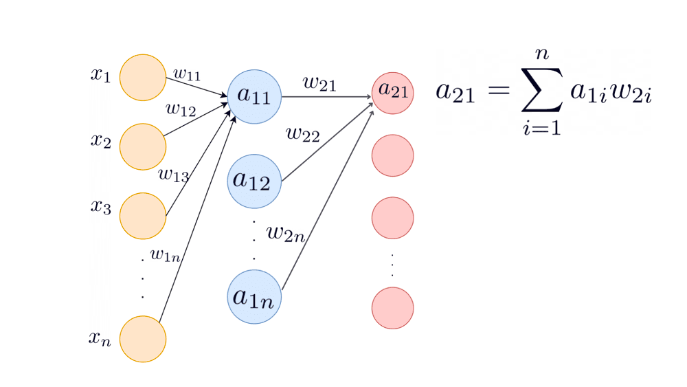
To compute the optimal variance, we’ll use as the first input to the first neuron in the second hidden layer, instead of . is proportional to , so we ignore the explicit effect of activations to simplify the derivation.
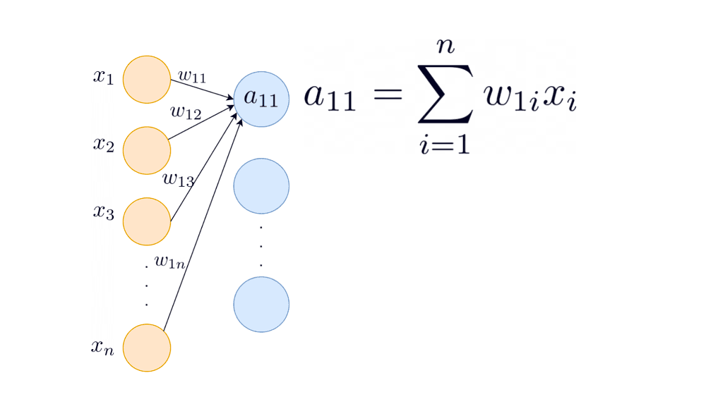
Weights flowing into the first neuron in the first hidden layer (Image by the author)
Assumption: The weights and inputs are uncorrelated.
Substituting and in the above equation:
Let’s compute the variance of in the second hidden layer.
By induction, the variance of input to neuron i in the hidden layer k is given by:
To ensure that the quantity n.Var(w) neither vanishes nor grows exponentially (leading to instability in the training process), we need n.Var(w) =1.
To achieve this, we can sample the weights from a standard normal distribution and scale them by a factor of .
X. Glorot and Y. Bengio proposed an improved weight initialization strategy named the Xavier or Glorot initialization [2] (after the researcher Xavier Glorot).
In a neural network, the number of weights that flow into each neuron in a neural network is called , and the number of weights that flow out of the neuron is called .
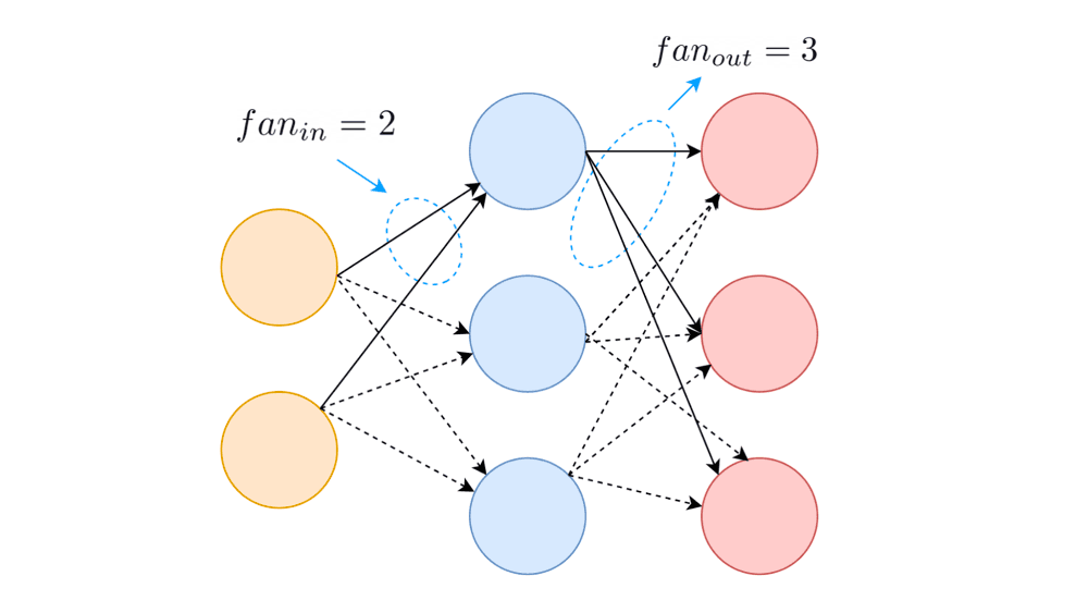
Explaining fan_in and fan_out (Image by the author)
When the weight distribution’s variance is set to , the activations neither vanish nor saturate during the forward pass.
However, during backpropagation, the gradients flow backward through the full network from the output layer to the input layer. We know that the of a neuron is the number of weights that flow out of the neuron into the next layer. But the of a particular neuron is also the number of paths through which gradients flow *into* it during backpropagation. Therefore, having the variance of the weights equal to helps overcome the problem of vanishing gradients.
To account for both the forward pass and backprop, we do the following: When computing the variance, instead of or , we consider the average of and .
A random variable that is uniformly distributed in an interval centered around zero has zero mean. So we can sample the weights from a uniform distribution with variance . But how do we find the endpoints of the interval?
A continuous random variable A that is uniformly distributed in the interval [-a,a] has zero mean and variance of .
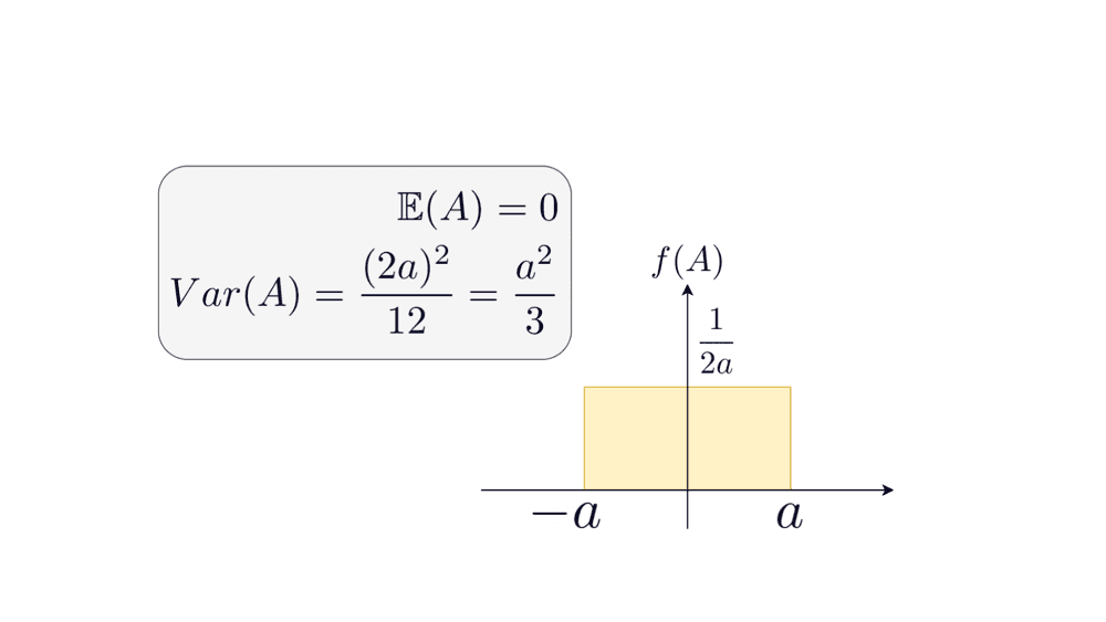
We know that the variance should be equal to ; we can work backward to find the endpoints of the interval.
To implement Glorot initialization in your deep learning models, you can use either the GlorotUniform or GlorotNormal class in the Keras initializers module. If you do not specify a kernel initializer when defining the model, it defaults to GlorotUniform.
GlorotNormal class initializes the weight tensors with samples from a truncated normal distribution with variance . When samples are drawn from a “truncated” normal distribution, samples that lie farther than two standard deviations away from the mean are discarded.GlorotUniform class initializes the weight tensors by sampling from a uniform distribution in the interval .It was found that Glorot initialization did not work for networks that used ReLU activations as the backflow of gradients was impacted [3].
But why does this happen?
Unlike the sigmoid and tanh activations, the ReLU function, which maps all negative inputs to zero: ReLU(x) = max(0,x), does not have a zero mean.
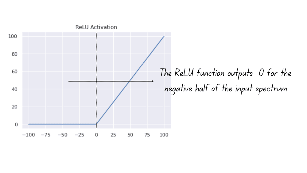
The ReLU function, therefore, outputs 0 for one-half of the input spectrum, whereas tanh and sigmoid activations give non-zero outputs for all values in the input space. Kaiming He et al. introduced a new initialization technique that takes this into account by introducing a factor of 2 when computing the variance [4].
As with Glorot initialization, we can also draw the weights from a uniform distribution for He initialization.
The Keras initializers module provides the HeNormal and HeUniform for He initialization.
HeNormal class initializes the weight tensors with samples drawn from a truncated normal distribution with zero mean and variance .HeUniform class initializes the weight tensors with samples drawn from a uniform distribution in the interval .Considering the when initializing weights, you can draw the weights from normal distribution with the following variance:
Equivalently, you may sample the initial weights from a uniform distribution with variance .
I hope this tutorial helped you understand the importance of weight initialization when training deep learning models.
When using deep learning in practice, you can experiment with weight initialization, regularization, and techniques such as batch normalization to improve the neural network’s training process. Happy learning and coding!
[1] G. E. Hinton, R. R. Salakhutdinov, Reducing the Dimensionality of Data with Neural Networks (2006), Sciences
[2] X. Glorot, Y. Bengio, Understanding the difficulty of training deep feedforward neural networks (2010), AISTATS 2010
[3] K. Kumar, On weight initialization in deep neural networks (2017)
[4] He et al., Delving Deep into Rectifiers: Surpassing Human-Level Performance on ImageNet Classification (2015), CVPR 2015
[5] Introduction to Statistical Signal Processing, Gray and Davisson
[6] Convex Optimization, Boyd and Vandenberghe
[7] Adaptive Methods and Non-convex Optimization, Advanced Machine Learning Systems, Cornell University, Fall 2021
[8] Layer weight initializers, keras.io
此内容由惯性聚合(RSS阅读器)自动聚合整理,仅供阅读参考。 原文来自 — 版权归原作者所有。