【转载】用OCTAVE实现一元线性回归的梯度下降算法

Posted on 2018-01-14 22:57 西瓜K菠萝阅读(377) 评论() 收藏举报

原文地址：http://www.cnblogs.com/KID-XiaoYuan/p/7247481.html

STEP1 PLOTTING THE DATA

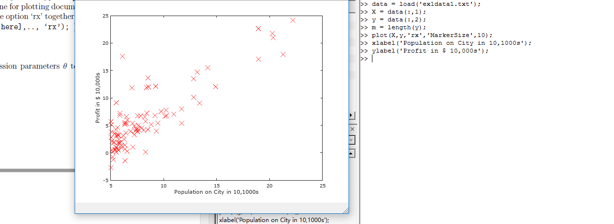
在处理数据之前，我们通常要了解数据，对于这次的数据集合，我们可以通过离散的点来描绘它，在一个2D的平面里把它画出来。

ex1data1.txt

我们把ex1data1中的内容读取到X变量和y变量中，用m表示数据长度。

data = load('ex1data1.txt');

X = data(:,1);

y = data(:,2);

m = length(y);

接下来通过图像描绘出来。

plot(x,y,'rx','MakerSize',10);

ylabel('Profit in $10,000s');

xlabel('Population of City in 10,000s');

　　现在我们得到图像如图所示，就是原始的数据的直观表示。

STEP2 GRADIENT DESCENT

现在，我们通过梯度下降法对参数θ进行线性回归。

依照我们之前所得出步骤方法

迭代更新

计算θ值函数：

function J = computeCost(X, y, theta)

m = length(y);

J = 0;

J = sum((X * theta - y).^2) / (2*m);

end

　　接下来是梯度下降函数

function [theta, J_history] = gradientDescent(X, y, theta, alpha, num_iters)

m = length(y);

J_history = zeros(num_iters, 1);

theta_s=theta;

for iter = 1:num_iters

theta(1) = theta(1) - alpha / m * sum(X * theta_s - y);

theta(2) = theta(2) - alpha / m * sum((X * theta_s - y) .* X(:,2));

theta_s=theta;

J_history(iter) = computeCost(X, y, theta);

end

J_history

end

绘图函数：

function plotData(x, y)

figure;

plot(x, y, 'rx', 'MarkerSize', 10);

ylabel('Profit in $10,000s');

xlabel('Population of City in 10,000s');

end

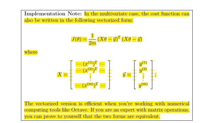
　　　　根据以上函数，我们进行线性回归：

100

101

102

103

104

105

106

107

108

109

110

111

112

113

114

115

116

117

118

119

120

<br>

fprintf('Running warmUpExercise ... \n');

fprintf('5x5 Identity Matrix: \n');

warmUpExercise()

fprintf('Program paused. Press enter to continue.\n');

pause;

fprintf('Plotting Data ...\n')

data = load('ex1data1.txt');

X = data(:, 1); y = data(:, 2);

m = length(y);

plotData(X, y);

fprintf('Program paused. Press enter to continue.\n');

pause;

fprintf('Running Gradient Descent ...\n')

X = [ones(m, 1), data(:,1)];

theta = zeros(2, 1);

iterations = 1500;

alpha = 0.01;

computeCost(X, y, theta)

theta = gradientDescent(X, y, theta, alpha, iterations);

fprintf('Theta found by gradient descent: ');

fprintf('%f %f \n', theta(1), theta(2));

hold on;

plot(X(:,2), X*theta, '-')

legend('Training data', 'Linear regression')

hold off

predict1 = [1, 3.5] *theta;

fprintf('For population = 35,000, we predict a profit of %f\n',...

predict1*10000);

predict2 = [1, 7] * theta;

fprintf('For population = 70,000, we predict a profit of %f\n',...

predict2*10000);

fprintf('Program paused. Press enter to continue.\n');

pause;

fprintf('Visualizing J(theta_0, theta_1) ...\n')

theta0_vals = linspace(-10, 10, 100);

theta1_vals = linspace(-1, 4, 100);

J_vals = zeros(length(theta0_vals), length(theta1_vals));

for i = 1:length(theta0_vals)

for j = 1:length(theta1_vals)

t = [theta0_vals(i); theta1_vals(j)];

J_vals(i,j) = computeCost(X, y, t);

end

J_vals = J_vals';

figure;

surf(theta0_vals, theta1_vals, J_vals)

xlabel('\theta_0'); ylabel('\theta_1');

figure;

contour(theta0_vals, theta1_vals, J_vals, logspace(-2, 3, 20))

xlabel('\theta_0'); ylabel('\theta_1');

hold on;

plot(theta(1), theta(2), 'rx', 'MarkerSize', 10, 'LineWidth', 2);

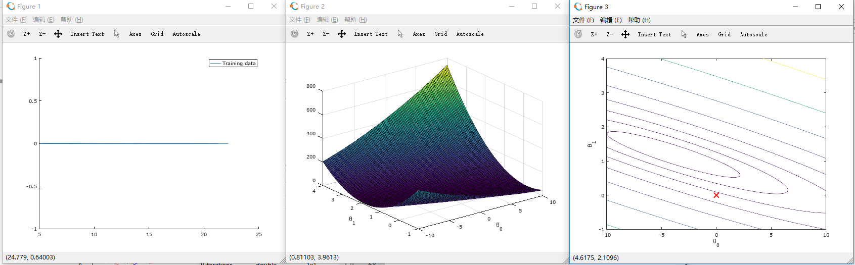
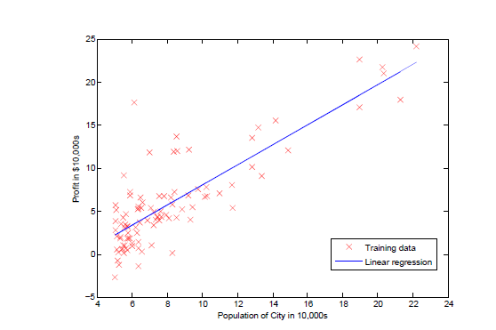
如图所示，绘制出线性回归函数。

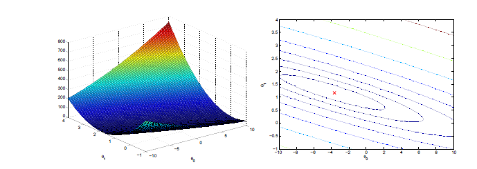
这时所绘制2D等高线图梯度下降表面图：

100

101

102

103

104

105

106

107

108

109

110

111

112

113

114

115

116

117

118

119

120

121

122

123

124

125

126

127

128

129

130

131

132

133

134

135

136

137

138

139

140

141

142

143

144

145

146

147

148

149

150

151

152

153

154

155

156

157

158

159

160

161

162

163

164

165

166

167

168

169

170

171

172

173

174

175

176

177

178

179

180

181

182

183

184

185

186

187

188

189

190

191

192

193

194

195

196

197

198

199

200

201

202

203

204

205

206

207

208

209

210

211

212

213

214

215

216

217

218

219

220

221

222

223

224

225

226

227

228

229

230

231

232

233

234

235

236

237

238

239

240

241

242

243

244

245

246

247

248

249

250

251

252

253

254

255

256

257

258

259

260

261

262

263

264

265

266

267

268

269

270

271

function [X_norm, mu, sigma] = featureNormalize(X)

X_norm = X;

mu = zeros(1, size(X, 2));

sigma = zeros(1, size(X, 2));

mu = mean(X);

sigma = std(X);

X_norm = (X - repmat(mu,size(X,1),1)) ./ repmat(sigma,size(X,1),1);

end

function [theta, J_history] = gradientDescentMulti(X, y, theta, alpha, num_iters)

m = length(y);

J_history = zeros(num_iters, 1);

for iter = 1:num_iters

theta = theta - alpha / m * X' * (X * theta - y);

J_history(iter) = computeCostMulti(X, y, theta);

end

function J = computeCostMulti(X, y, theta)

m = length(y);

J = 0;

J = sum((X * theta - y).^2) / (2*m);

end

function [theta] = normalEqn(X, y)

theta = zeros(size(X, 2), 1);

theta = pinv( X' * X ) * X' * y;

end

clear ; close all; clc

fprintf('Loading data ...\n');

data = load('ex1data2.txt');

X = data(:, 1:2);

y = data(:, 3);

m = length(y);

fprintf('First 10 examples from the dataset: \n');

fprintf(' x = [%.0f %.0f], y = %.0f \n', [X(1:10,:) y(1:10,:)]');

fprintf('Program paused. Press enter to continue.\n');

pause;

fprintf('Normalizing Features ...\n');

[X mu sigma] = featureNormalize(X);

X = [ones(m, 1) X];

fprintf('Running gradient descent ...\n');

alpha = 0.01;

num_iters = 8500;

theta = zeros(3, 1);

[theta, J_history] = gradientDescentMulti(X, y, theta, alpha, num_iters);

figure;

plot(1:numel(J_history), J_history, '-b', 'LineWidth', 2);

xlabel('Number of iterations');

ylabel('Cost J');

fprintf('Theta computed from gradient descent: \n');

fprintf(' %f \n', theta);

fprintf('\n');

price = [1 (([1650 3]-mu) ./ sigma)] * theta ;

fprintf(['Predicted price of a 1650 sq-ft, 3 br house ' ...

'(using gradient descent):\n $%f\n'], price);

fprintf('Program paused. Press enter to continue.\n');

pause;

fprintf('Solving with normal equations...\n');

data = csvread('ex1data2.txt');

X = data(:, 1:2);

y = data(:, 3);

m = length(y);

X = [ones(m, 1) X];

theta = normalEqn(X, y);

fprintf('Theta computed from the normal equations: \n');

fprintf(' %f \n', theta);

fprintf('\n');

price = [1 1650 3] * theta ;

fprintf(['Predicted price of a 1650 sq-ft, 3 br house ' ...

'(using normal equations):\n $%f\n'], price);

　　处理前：

处理后：

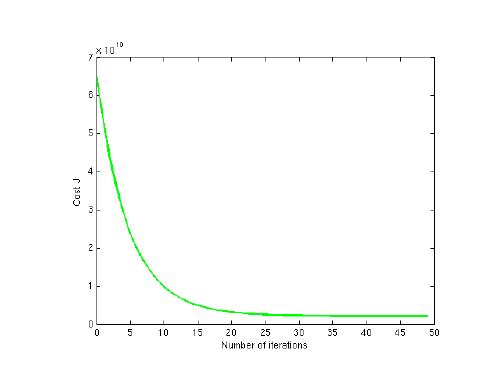
回归过程如图所示：

至此，我们通过梯度下降法解决了此问题，我们还可以通过之前所说的数学方法来解决，但是对于数据太大的情况（通常大于10000），我们就会通过梯度下降法来解决了

　　根据以上函数，我们进行线性回归：

推荐订阅源

博客园 - 西瓜K菠萝

STEP1 PLOTTING THE DATA

STEP2 GRADIENT DESCENT