推荐订阅源

逻辑回归（Logistic Regression）是一种广泛应用于分类问题的统计学习方法，尽管名字中带有"回归"，但它实际上是一种用于二分类或多分类问题的算法。

逻辑回归通过使用逻辑函数（也称为 Sigmoid 函数）将线性回归的输出映射到 0 和 1 之间，从而预测某个事件发生的概率。

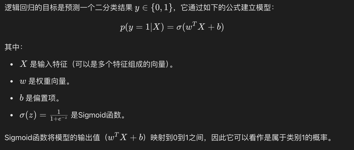
 逻辑回归的损失函数是对数损失函数（Log Loss）

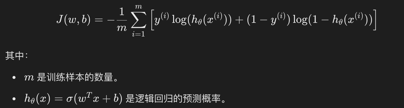
 逻辑回归通常也使用梯度下降法来优化损失函数，求解参数 w 和 b

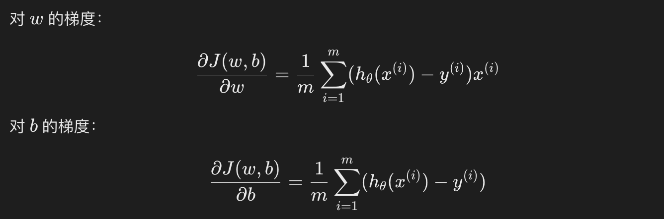
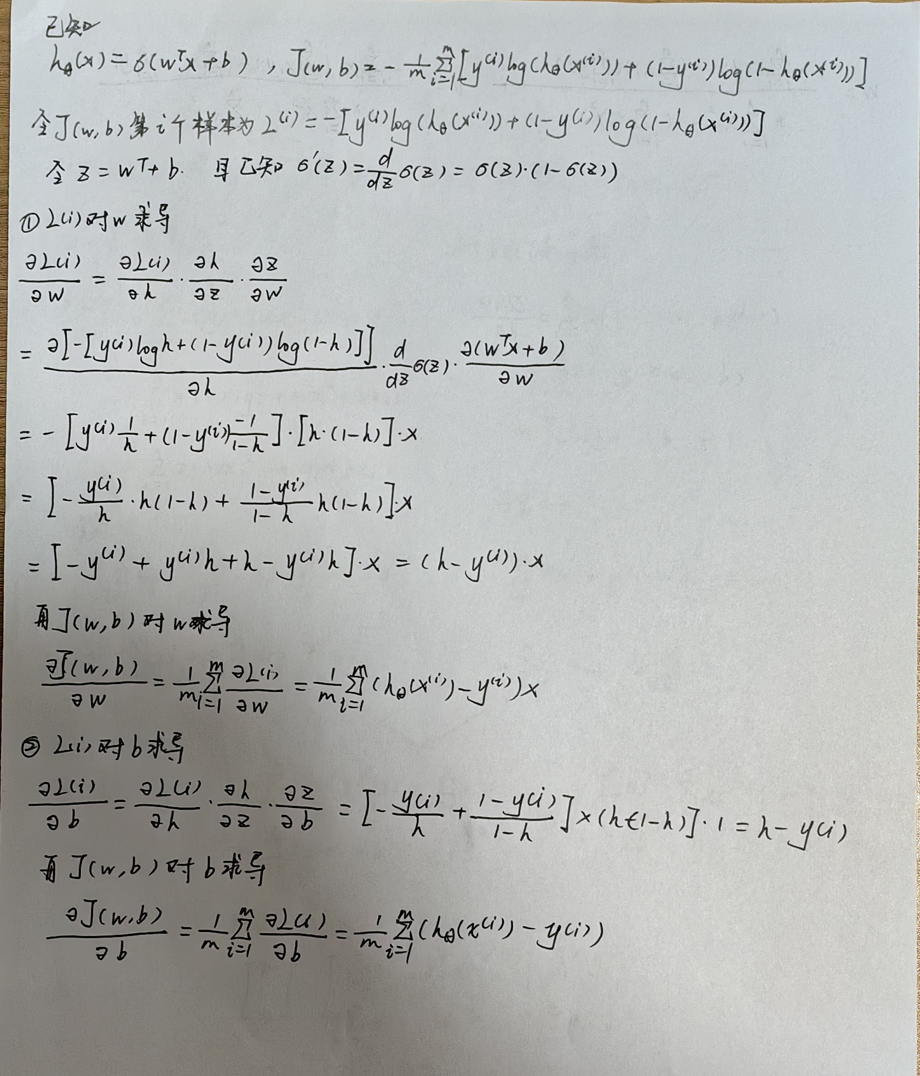
求解过程：

 使用 Python 和 Scikit-learn 库来实现一个简单的逻辑回归模型。

import numpy as np
import matplotlib.pyplot as plt
from sklearn.datasets import load_iris
from sklearn.model_selection import train_test_split
from sklearn.linear_model import LogisticRegression
from sklearn.metrics import accuracy_score, confusion_matrix, classification_report

# 加载数据集
iris = load_iris()
X = iris.data[:, :2]  # 只使用前两个特征
y = (iris.target != 0) * 1  # 将目标转化为二分类问题

# 划分训练集和测试集
X_train, X_test, y_train, y_test = train_test_split(X, y, test_size=0.3, random_state=42)


# 创建逻辑回归模型
model = LogisticRegression()

# 训练模型
model.fit(X_train, y_train)

# 预测测试集
y_pred = model.predict(X_test)

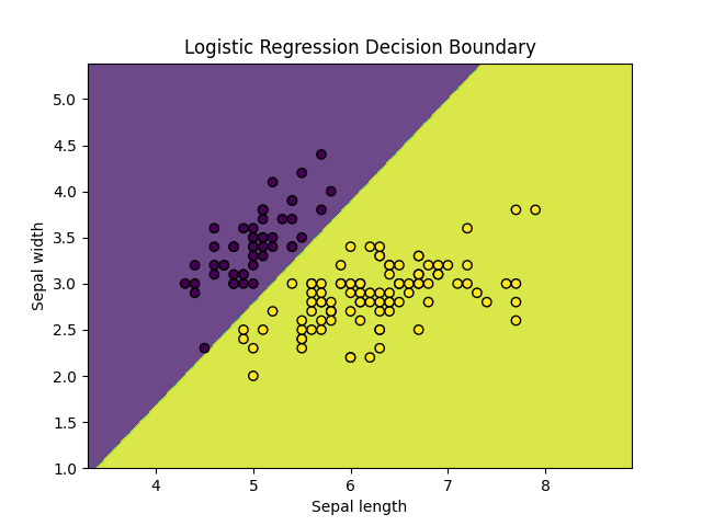
# 可视化决策边界
x_min, x_max = X[:, 0].min() - 1, X[:, 0].max() + 1
y_min, y_max = X[:, 1].min() - 1, X[:, 1].max() + 1
xx, yy = np.meshgrid(np.arange(x_min, x_max, 0.01),
                     np.arange(y_min, y_max, 0.01))

Z = model.predict(np.c_[xx.ravel(), yy.ravel()])
Z = Z.reshape(xx.shape)

plt.contourf(xx, yy, Z, alpha=0.8)
plt.scatter(X[:, 0], X[:, 1], c=y, edgecolors='k', marker='o')
plt.xlabel('Sepal length')
plt.ylabel('Sepal width')
plt.title('Logistic Regression Decision Boundary')
plt.show()