







 Summarize this articleHere’s what you need to know:
At the dawn of experimentation, statisticians provided a very basic framework for statistical inference in A/B testing scenarios. Still commonly used today, The Frequentist Approach, under which Hypothesis Testing was developed, allowed the industry to further investigate theories of behavior and determine whether there is enough statistical evidence to support a specific theory.
Later, differences in how to most effectively interpret probability would give rise to a new, Bayesian Approach – a method many say is less restrictive, highly intuitive, and more reliable (a sentiment also shared by us at Dynamic Yield). For the purpose of this post, I will dive into the numbers behind the Frequentists school of thought, performing the appropriate derivations where necessary.
At a very high level, when performing a traditional A/B test, one starts with a hypothesis – a predictive statement about the impact of a change. Following this, a sample size is calculated to achieve Statistical Significance (95%), the traffic is split among the variations, results measured, and a conclusion reached, either validating or failing to validate the original hypothesis.
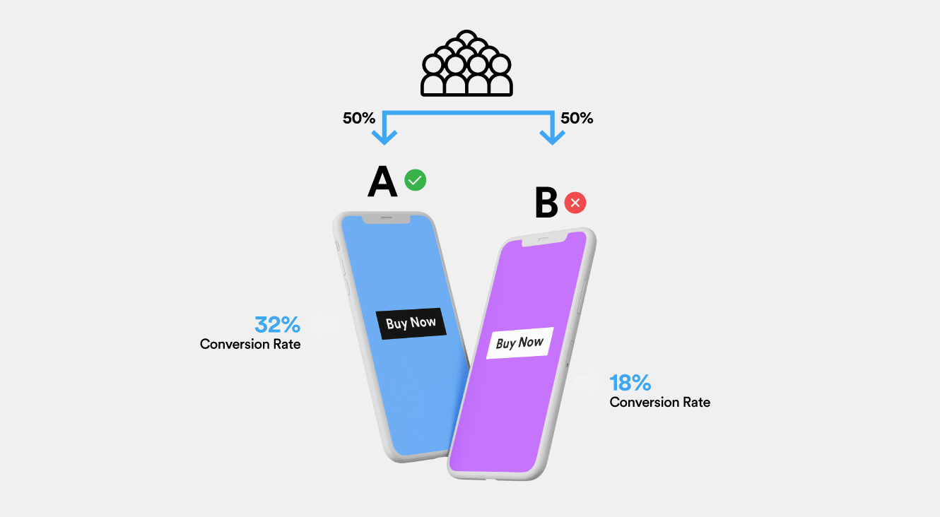
Reaching a hypothesis is usually done after an internal brainstorming session, or discovered through focus group research. I will talk about calculating sample size later. The third step in the process, measuring the results, is where things start to get complicated.
If you had to arrive at a click-through rate for each variation, can you show each variation to a single user, calculate the click-through rate, and conclude which variation is better? Obviously not!
We know intuitively that one click out of 10 impressions is not as reliable as ten clicks out of 100, even though both scenarios have the same click-through rates. So, extending this logic, in an ideal scenario, one has to run the test for an infinite amount of time, reach the true conversion rates of both variations, and conclude the test with 100% confidence.
Since this is not an option, we work with Likelihood functions, answering the question: which click-through rate of a variation is closest to the ‘true’ click-through rate?
When you initially start collecting data from your variations, it’s normal to see numbers falling all over the place. So, how can one find a single value that represents the conversion rate of the variation? By finding out the sample mean estimate.
The data collected during the experiment can usually be characterized by an underlying distribution. For example, Gaussian / normal distribution, if you are measuring the height of students in a class, or Bernoulli, if you are mapping a binary variable like a coin toss.
In our case, the click-through rate most likely follows a Gaussian distribution. Gaussian distribution is defined by two parameters: mean (μ) and variance ( ² ).

The wider the distribution is, the more far off the sample data is from each other. As you can see, there can be many Gaussian distributions with different mean values that can possibly represent the underlying data.
But there is only one Gaussian distribution which maximizes the probability of seeing the observations – the Maximum Likelihood. The mean value at which this ‘maximum likelihood estimate’ occurs is the ‘sample mean estimate’ we are after. This sample mean estimate value will be the closest to the ‘ideal conversion rate’ given the data collected for a variation.

Let’s go back to school and try to derive the sample mean estimate. If you are not interested in the derivation, you can scroll to the bottom of this section for the concluding formula.
I am working with a Gaussian distribution first, here. Later, we will do the same for a Bernoulli.
The Probability Density Function of a Gaussian is:

If you have a Gaussian distribution with a mean and variance and want to calculate the probability that a particular value ‘X’ is going to occur, then you just fill the equation with the value of X and get the probability of that value.
Extending this logic, if one wants to find the joint probability of all the samples collected in an experiment, then because the samples are independent and identically distributed (IID), we can just multiply the probabilities of individual samples as follows:

This likelihood function answers the main question: what’s the probability of seeing these data points given the mean value μ?

Maximum Likelihood maximizes the value of the likelihood function, answering the most critical question: what value of μ maximizes the probability of the data in the samples I am seeing?
In calculus, to maximize a function with respect to a variable, we find the derivative:
dp/dμ = 0, solving for μ
Since the Gaussian is an exponential function, the derivative would, again, be an exponential. To avoid this, we take Log on both sides, reducing the exponential to linear values (the Log is a monotonically increasing function, just like the exponential):




Now, finding the derivative of the log-likelihood with respect to μ, we get:
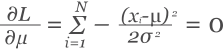
Therefore, the sample mean estimate is:

The same logic can be applied for a Bernoulli.
The likelihood function of a Bernoulli distribution is:

Following a similar process, taking Log on both sides and performing a derivative w.r.t p, we get the sample mean estimate of a Bernoulli as:


Where xi represents the number of times the events occurred / did not occur. So, the sample mean estimate is similar for both Gaussian and Bernoulli distribution, and both have a very glaring problem.
As seen before, the sample mean estimate boils down to:

Let’s say you collect two click-through rates. For example, 10.5 % & 9.5 %, and apply the formula to calculate sample mean estimate:
(10.5 + 9.5) / 2
At 10%, does it answer how confident you can be in your estimate? Does it quantify the uncertainty? Does it tell you how close or far you are to understanding the ‘true’ click-through rate?
Clearly not, which is why we work with Confidence Intervals and P-Values – so that we can quantify the uncertainty around the data collected by incorporating the number of samples into the equation.
Having calculated the sample mean estimate ( ∧μ ), we can conclude with 95% confidence that the ‘true’ click-through rate would lie between:

Where tα = the test-statistic at a 95% confidence level and N-1 degrees of freedom (this is a readily available pre-calculated number).
δ = the sample standard deviation
N = the sample size
Now that we have established confidence intervals around our observed data in a test, how do we extend that to our Hypothesis Testing and conclude if our hypothesis is true?
To do that:
We calculate the test statistic as under:

Map the test-statistic to a p-value
Reject the hypothesis if the value is above the threshold Pcritical value
Let’s break down each step to understand better.
Step 1: The higher the difference between the sample mean estimates of the variations, the higher the test-statistic. Intuitively, the higher the difference, the clearer the winner is, so a rule of thumb is that the Absolute Value of the test-statistic should always be higher.
Step 2: The test-statistic is a point value on a normal distribution, which shows how far off (in no. of standard deviations) from the mean the test-statistic is. To convert the point estimate into a probability, we need the area under the curve, or mathematically speaking, the cumulative density function. We can do the integral of the t-distribution or the Gaussian distribution and find out how much area under the curve is covered by the test-statistic – this value is called the p-value. Thankfully these numbers are pre-calculated and publicly available, so we do not have to go over the nitty-gritty details
Step 3: Once p-value is known, interpreting it is pretty straight forward. If the calculated p-value is less than the Pcritical value, you set is as the threshold for rejecting the null hypothesis, and if it is more than the Pcritical value, then you fail to reject the null hypothesis. This does not mean you accept that the null hypothesis is true. More on this later.
A very convoluted metric that can lead to a lot of confusion, the official definition of p-value is as follows:
“The probability that, when the null hypothesis is true, the statistical summary (such as the sample mean difference between two groups) would be equal to, or more extreme than, the actual observed results.”
To explain, let’s say you start with a hypothesis that both women and men are of the same height. You collect some data, calculate sample mean heights and find 1.9 meters for men and 1.7 meters for women, with a p-value of 0.03. This p-value tells you IF the null hypothesis is true, what the probability is you would see the difference (or greater) as measured in your samples.
In other words, IF, in fact, women and men were of the same height, then the probability of us seeing a difference of 0.2 in the mean values between them is 3%. We’d, therefore, reject the hypothesis, as this is extremely rare, and say the alternate is true. The value at which you say the probability is rare enough is the critical value of p. This is usually 0.05 or 0.01, so we are saying you can live with making an incorrect conclusion 5% of the time.
Now, time to talk about errors.
Attempting to logically interpret an A/B test situation, there are two types of errors that are theoretically possible:
Falsely reject a true null hypothesis (type I or alpha) or
Fail to reject a false null hypothesis (type II or beta)
The table below gives a nice overview:
| Decision -> Reality | Reject Ho | Fail to Reject Ho |
| Ho is True | False Positive (Type I) | True Negative |
| H1 is True | True Positive | False Negative (Type II) |
It’s easier to think of errors in terms of False Positives and False Negatives. A false positive is when you’ve identified a non-existing relationship.
How does such a thing happen?
Let’s say you start an A/B test with a p-value of 0.01. A typical A/B test has a progression of p-value like below:

The blue line shows p-value and the green, significance level. As you can imagine, concluding the test before the sample size is large enough would be the wrong decision, resulting in one trying to find evidence when there is none. This is the reason why it’s advised not to ‘peek’ at a running A/B test, for it may lead to incorrect decision-making based on inappropriate data.
Achieving significance is not ‘incremental’ by nature in traditional A/B testing. You do not see the results gradually improving over time; you calculate a sample size, refrain from peeking until it’s reached, and then try to draw a conclusion once the estimated sample threshold has been hit.
Failure to do so could be extremely problematic. Whether you are running a flash sale with limited time for iterations or you’re a medical company trying to solve a life-threatening disease – you would not be able to stop your traditional A/B test or treatment halfway through and start curing people. You’d have to wait until the test was properly completed out of fear of producing a false positive.
When running a traditional A/B test where one variation is clearly outperforming another, the losing variation is still shown to a large audience until the statistical significance is reached. While allowing for confident winner-declaration, the time spent waiting can result in a loss of potential business.
In an ideal world, you should be able to drop traffic to the losing variation and maximize returns with the winning variation. To provide the losing variation an opportunity to take the lead, we assign a bare minimum percentage of the traffic to it (called Epsilon) and exploit the winning variation. Thus the term ‘Explore vs. Exploit’ (also called ‘epsilon-greedy’ in some circles) has come to be, which addresses how much time is “wasted” on learning as opposed to taking advantage of what is already learned. This feature is nearly impossible in a traditional A/B test, unless you are hell-bent on producing false positives.
Recapping everything that has been laid out so far:
Traditional A/B testing can quickly get out of hand with observations including a high standard deviation due to imbalances in the scales tilting the sample mean estimate.
A marginally high standard deviation in the sample population would require a larger number of samples to reach acceptable significance levels.
Achieving significance is not ‘incremental’ by nature in traditional A/B testing. A ‘no peeking’ approach should be followed until the completion of a test.
There is always the possibility of a ‘false positive’ or type-1 error, especially if you hurry the test or peek at the results too early.
An Explore-Exploit strategy is not possible, and therefore you leave money on the table by continuing to serve a losing variation.
P-value is highly convoluted and not intuitive.
For all of these reasons, we at Dynamic Yield prefer the Bayesian approach to A/B testing. Click to read more on exactly how going Bayesian overcomes some of the issues we’ve outlined above presented in traditional A/B testing.
此内容由惯性聚合(RSS阅读器)自动聚合整理,仅供阅读参考。 原文来自 — 版权归原作者所有。