

惯性聚合 高效追踪和阅读你感兴趣的博客、新闻、科技资讯
阅读原文 在惯性聚合中打开

推荐订阅源

B
Blog
V
Vulnerabilities – Threatpost
Apple Machine Learning Research
V
V2EX
博客园 - 叶小钗
阮一峰的网络日志
阮一峰的网络日志
人人都是产品经理
人人都是产品经理
Latest news
Latest news
博客园 - 三生石上(FineUI控件)
美团技术团队
aimingoo的专栏
aimingoo的专栏
Google Online Security Blog
Security Archives - TechRepublic
T
Threatpost
Y
Y Combinator Blog
T
Tailwind CSS Blog
CTFtime.org: upcoming CTF events
A
Arctic Wolf
C
Cyber Attacks, Cyber Crime and Cyber Security
小众软件
小众软件
Recent Commits to openclaw:main
T
Tenable Blog
W
WeLiveSecurity
L
LINUX DO - 热门话题
D
Docker
Cyberwarzone
Cyberwarzone
量子位
A
About on SuperTechFans
The Last Watchdog
The Last Watchdog
雷峰网
雷峰网
C
CERT Recently Published Vulnerability Notes
P
Palo Alto Networks Blog
The Hacker News
The Hacker News
Blog — PlanetScale
Blog — PlanetScale
P
Proofpoint News Feed
OSCHINA 社区最新新闻
OSCHINA 社区最新新闻
F
Full Disclosure
The Cloudflare Blog
T
The Blog of Author Tim Ferriss
T
The Exploit Database - CXSecurity.com
Engineering at Meta
Engineering at Meta
O
OpenAI News
Hacker News - Newest:
Hacker News - Newest: "LLM"
Scott Helme
Scott Helme
IT之家
IT之家
S
Secure Thoughts
MongoDB | Blog
MongoDB | Blog
L
Lohrmann on Cybersecurity
博客园 - 司徒正美
Google DeepMind News

Hugging Face - Blog

Waypoint-1.5: Higher-Fidelity Interactive Worlds for Everyday GPUs ALTK‑Evolve: On‑the‑Job Learning for AI Agents Safetensors is Joining the PyTorch Foundation Holo3: Breaking the Computer Use Frontier Any Custom Frontend with Gradio's Backend A New Framework for Evaluating Voice Agents (EVA) Bringing Robotics AI to Embedded Platforms: Dataset Recording, VLA Fine‑Tuning, and On‑Device Optimizations One-Shot Any Web App with Gradio's gr.HTML CUGA on Hugging Face: Democratizing Configurable AI Agents New in llama.cpp: Model Management Building Deep Research: How we Achieved State of the Art OVHcloud on Hugging Face Inference Providers 🔥 20x Faster TRL Fine-tuning with RapidFire AI Building for an Open Future - our new partnership with Google Cloud Aligning to What? Rethinking Agent Generalization in MiniMax M2 Building a Healthcare Robot from Simulation to Deployment with NVIDIA Isaac Sentence Transformers is joining Hugging Face! Unlock the power of images with AI Sheets Supercharge your OCR Pipelines with Open Models Google Cloud C4 Brings a 70% TCO improvement on GPT OSS with Intel and Hugging Face Get your VLM running in 3 simple steps on Intel CPUs Nemotron-Personas-India: Synthesized Data for Sovereign AI Introducing RTEB: A New Standard for Retrieval Evaluation Accelerating Qwen3-8B Agent on Intel® Core™ Ultra with Depth-Pruned Draft Models VibeGame: Exploring Vibe Coding Games Nemotron-Personas-Japan: ソブリン AI のための合成データセット Swift Transformers Reaches 1.0 – and Looks to the Future Smol2Operator: Post-Training GUI Agents for Computer Use SyGra: The One-Stop Framework for Building Data for LLMs and SLMs Gaia2 and ARE: Empowering the community to study agents Scaleway on Hugging Face Inference Providers 🔥 Democratizing AI Safety with RiskRubric.ai Public AI on Hugging Face Inference Providers 🔥 `LeRobotDataset:v3.0`: Bringing large-scale datasets to `lerobot` Visible Watermarking with Gradio Introducing the Palmyra-mini family: Powerful, lightweight, and ready to reason! Tricks from OpenAI gpt-oss YOU 🫵 can use with transformers Fine-tune Any LLM from the Hugging Face Hub with Together AI Jupyter Agents: training LLMs to reason with notebooks mmBERT: ModernBERT goes Multilingual Welcome EmbeddingGemma, Google's new efficient embedding model SAIR: Accelerating Pharma R&D with AI-Powered Structural Intelligence Make your ZeroGPU Spaces go brrr with ahead-of-time compilation NVIDIA Releases 6 Million Multi-Lingual Reasoning Dataset Generate Images with Claude and Hugging Face From Zero to GPU: A Guide to Building and Scaling Production-Ready CUDA Kernels MCP for Research: How to Connect AI to Research Tools Kimina-Prover-RL Arm & ExecuTorch 0.7: Bringing Generative AI to the masses Neural Super Sampling is here! TextQuests: How Good are LLMs at Text-Based Video Games? 🇵🇭 FilBench - Can LLMs Understand and Generate Filipino? Introducing AI Sheets: a tool to work with datasets using open AI models! Accelerate ND-Parallel: A guide to Efficient Multi-GPU Training Vision Language Model Alignment in TRL ⚡️ Welcome GPT OSS, the new open-source model family from OpenAI! Measuring Open-Source Llama Nemotron Models on DeepResearch Bench 📚 3LM: A Benchmark for Arabic LLMs in STEM and Code Implementing MCP Servers in Python: An AI Shopping Assistant with Gradio Introducing Trackio: A Lightweight Experiment Tracking Library from Hugging Face Say hello to `hf`: a faster, friendlier Hugging Face CLI ✨ Parquet Content-Defined Chunking TimeScope: How Long Can Your Video Large Multimodal Model Go? Fast LoRA inference for Flux with Diffusers and PEFT Accelerate a World of LLMs on Hugging Face with NVIDIA NIM Arc Virtual Cell Challenge: A Primer Consilium: When Multiple LLMs Collaborate Back to The Future: Evaluating AI Agents on Predicting Future Events Five Big Improvements to Gradio MCP Servers Ettin Suite: SoTA Paired Encoders and Decoders Migrating the Hub from Git LFS to Xet Kimina-Prover: Applying Test-time RL Search on Large Formal Reasoning Models Asynchronous Robot Inference: Decoupling Action Prediction and Execution ScreenEnv: Deploy your full stack Desktop Agent Building the Hugging Face MCP Server Reachy Mini - The Open-Source Robot for Today's and Tomorrow's AI Builders Creating custom kernels for the AMD MI300 Upskill your LLMs With Gradio MCP Servers SmolLM3: smol, multilingual, long-context reasoner Three Mighty Alerts Supporting Hugging Face’s Production Infrastructure Efficient MultiModal Data Pipeline Announcing NeurIPS 2025 E2LM Competition: Early Training Evaluation of Language Models Training and Finetuning Sparse Embedding Models with Sentence Transformers Welcome the NVIDIA Llama Nemotron Nano VLM to Hugging Face Hub Gemma 3n fully available in the open-source ecosystem! Transformers backend integration in SGLang (LoRA) Fine-Tuning FLUX.1-dev on Consumer Hardware Groq on Hugging Face Inference Providers 🔥 How Long Prompts Block Other Requests - Optimizing LLM Performance Learn the Hugging Face Kernel Hub in 5 Minutes Convert Transformers to ONNX with Hugging Face Optimum Intel and Hugging Face Partner to Democratize Machine Learning Hardware Acceleration Director of Machine Learning Insights [Part 3: Finance Edition] The Annotated Diffusion Model Deep Q-Learning with Space Invaders Graphcore and Hugging Face Launch New Lineup of IPU-Ready Transformers Introducing Pull Requests and Discussions 🥳 Efficient Table Pre-training without Real Data: An Introduction to TAPEX An Introduction to Q-Learning Part 2/2 How Sempre Health is leveraging the Expert Acceleration Program to accelerate their ML roadmap
Introduction to Graph Machine Learning
Clémentine Fourrier · 2023-01-03 · via Hugging Face - Blog

Back to Articles

Clémentine Fourrier's avatar

This article is also available in Chinese 简体中文.

In this blog post, we cover the basics of graph machine learning.

We first study what graphs are, why they are used, and how best to represent them. We then cover briefly how people learn on graphs, from pre-neural methods (exploring graph features at the same time) to what are commonly called Graph Neural Networks. Lastly, we peek into the world of Transformers for graphs.

Graphs

What is a graph?

In its essence, a graph is a description of items linked by relations.

Examples of graphs include social networks (Twitter, Mastodon, any citation networks linking papers and authors), molecules, knowledge graphs (such as UML diagrams, encyclopedias, and any website with hyperlinks between its pages), sentences expressed as their syntactic trees, any 3D mesh, and more! It is, therefore, not hyperbolic to say that graphs are everywhere.

The items of a graph (or network) are called its nodes (or vertices), and their connections its edges (or links). For example, in a social network, nodes are users and edges their connections; in a molecule, nodes are atoms and edges their molecular bond.

  • A graph with either typed nodes or typed edges is called heterogeneous (example: citation networks with items that can be either papers or authors have typed nodes, and XML diagram where relations are typed have typed edges). It cannot be represented solely through its topology, it needs additional information. This post focuses on homogeneous graphs.
  • A graph can also be directed (like a follower network, where A follows B does not imply B follows A) or undirected (like a molecule, where the relation between atoms goes both ways). Edges can connect different nodes or one node to itself (self-edges), but not all nodes need to be connected.

If you want to use your data, you must first consider its best characterisation (homogeneous/heterogeneous, directed/undirected, and so on).

What are graphs used for?

Let's look at a panel of possible tasks we can do on graphs.

At the graph level, the main tasks are:

  • graph generation, used in drug discovery to generate new plausible molecules,
  • graph evolution (given a graph, predict how it will evolve over time), used in physics to predict the evolution of systems
  • graph level prediction (categorisation or regression tasks from graphs), such as predicting the toxicity of molecules.

At the node level, it's usually a node property prediction. For example, Alphafold uses node property prediction to predict the 3D coordinates of atoms given the overall graph of the molecule, and therefore predict how molecules get folded in 3D space, a hard bio-chemistry problem.

At the edge level, it's either edge property prediction or missing edge prediction. Edge property prediction helps drug side effect prediction predict adverse side effects given a pair of drugs. Missing edge prediction is used in recommendation systems to predict whether two nodes in a graph are related.

It is also possible to work at the sub-graph level on community detection or subgraph property prediction. Social networks use community detection to determine how people are connected. Subgraph property prediction can be found in itinerary systems (such as Google Maps) to predict estimated times of arrival.

Working on these tasks can be done in two ways.

When you want to predict the evolution of a specific graph, you work in a transductive setting, where everything (training, validation, and testing) is done on the same single graph. If this is your setup, be careful! Creating train/eval/test datasets from a single graph is not trivial. However, a lot of the work is done using different graphs (separate train/eval/test splits), which is called an inductive setting.

How do we represent graphs?

The common ways to represent a graph to process and operate it are either:

  • as the set of all its edges (possibly complemented with the set of all its nodes)
  • or as the adjacency matrix between all its nodes. An adjacency matrix is a square matrix (of node size * node size) that indicates which nodes are directly connected to which others (where (A_{ij} = 1) if (n_i) and (n_j) are connected, else 0). Note: most graphs are not densely connected and therefore have sparse adjacency matrices, which can make computations harder.

However, though these representations seem familiar, do not be fooled!

Graphs are very different from typical objects used in ML because their topology is more complex than just "a sequence" (such as text and audio) or "an ordered grid" (images and videos, for example)): even if they can be represented as lists or matrices, their representation should not be considered an ordered object!

But what does this mean? If you have a sentence and shuffle its words, you create a new sentence. If you have an image and rearrange its columns, you create a new image.
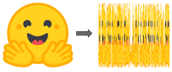
On the left, the Hugging Face logo - on the right, a shuffled Hugging Face logo, which is quite a different new image.

This is not the case for a graph: if you shuffle its edge list or the columns of its adjacency matrix, it is still the same graph. (We explain this more formally a bit lower, look for permutation invariance).
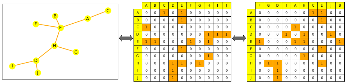
On the left, a small graph (nodes in yellow, edges in orange). In the centre, its adjacency matrix, with columns and rows ordered in the alphabetical node order: on the row for node A (first row), we can read that it is connected to E and C. On the right, a shuffled adjacency matrix (the columns are no longer sorted alphabetically), which is also a valid representation of the graph: A is still connected to E and C.

Graph representations through ML

The usual process to work on graphs with machine learning is first to generate a meaningful representation for your items of interest (nodes, edges, or full graphs depending on your task), then to use these to train a predictor for your target task. We want (as in other modalities) to constrain the mathematical representations of your objects so that similar objects are mathematically close. However, this similarity is hard to define strictly in graph ML: for example, are two nodes more similar when they have the same labels or the same neighbours?

Note: In the following sections, we will focus on generating node representations. Once you have node-level representations, it is possible to obtain edge or graph-level information. For edge-level information, you can concatenate node pair representations or do a dot product. For graph-level information, it is possible to do a global pooling (average, sum, etc.) on the concatenated tensor of all the node-level representations. Still, it will smooth and lose information over the graph -- a recursive hierarchical pooling can make more sense, or add a virtual node, connected to all other nodes in the graph, and use its representation as the overall graph representation.

Pre-neural approaches

Simply using engineered features

Before neural networks, graphs and their items of interest could be represented as combinations of features, in a task-specific fashion. Now, these features are still used for data augmentation and semi-supervised learning, though more complex feature generation methods exist; it can be essential to find how best to provide them to your network depending on your task.

Node-level features can give information about importance (how important is this node for the graph?) and/or structure based (what is the shape of the graph around the node?), and can be combined.

The node centrality measures the node importance in the graph. It can be computed recursively by summing the centrality of each node’s neighbours until convergence, or through shortest distance measures between nodes, for example. The node degree is the quantity of direct neighbours it has. The clustering coefficient measures how connected the node neighbours are. Graphlets degree vectors count how many different graphlets are rooted at a given node, where graphlets are all the mini graphs you can create with a given number of connected nodes (with three connected nodes, you can have a line with two edges, or a triangle with three edges).
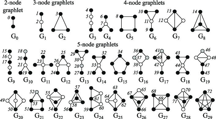
The 2-to 5-node graphlets (Pržulj, 2007)

Edge-level features complement the representation with more detailed information about the connectedness of the nodes, and include the shortest distance between two nodes, their common neighbours, and their Katz index (which is the number of possible walks of up to a certain length between two nodes - it can be computed directly from the adjacency matrix).

Graph level features contain high-level information about graph similarity and specificities. Total graphlet counts, though computationally expensive, provide information about the shape of sub-graphs. Kernel methods measure similarity between graphs through different "bag of nodes" methods (similar to bag of words).

Walk-based approaches

Walk-based approaches use the probability of visiting a node j from a node i on a random walk to define similarity metrics; these approaches combine both local and global information. Node2Vec, for example, simulates random walks between nodes of a graph, then processes these walks with a skip-gram, much like we would do with words in sentences, to compute embeddings. These approaches can also be used to accelerate computations of the Page Rank method, which assigns an importance score to each node (based on its connectivity to other nodes, evaluated as its frequency of visit by random walk, for example).

However, these methods have limits: they cannot obtain embeddings for new nodes, do not capture structural similarity between nodes finely, and cannot use added features.

Graph Neural Networks

Neural networks can generalise to unseen data. Given the representation constraints we evoked earlier, what should a good neural network be to work on graphs?

It should:

  • be permutation invariant:
    • Equation: f(P(G))=f(G)f(P(G))=f(G) with f the network, P the permutation function, G the graph
    • Explanation: the representation of a graph and its permutations should be the same after going through the network
  • be permutation equivariant
    • Equation: P(f(G))=f(P(G))P(f(G))=f(P(G)) with f the network, P the permutation function, G the graph
    • Explanation: permuting the nodes before passing them to the network should be equivalent to permuting their representations

Typical neural networks, such as RNNs or CNNs are not permutation invariant. A new architecture, the Graph Neural Network, was therefore introduced (initially as a state-based machine).

A GNN is made of successive layers. A GNN layer represents a node as the combination (aggregation) of the representations of its neighbours and itself from the previous layer (message passing), plus usually an activation to add some nonlinearity.

Comparison to other models: A CNN can be seen as a GNN with fixed neighbour sizes (through the sliding window) and ordering (it is not permutation equivariant). A Transformer without positional embeddings can be seen as a GNN on a fully-connected input graph.

Aggregation and message passing

There are many ways to aggregate messages from neighbour nodes, summing, averaging, for example. Some notable works following this idea include:

  • Graph Convolutional Networks averages the normalised representation of the neighbours for a node (most GNNs are actually GCNs);
  • Graph Attention Networks learn to weigh the different neighbours based on their importance (like transformers);
  • GraphSAGE samples neighbours at different hops before aggregating their information in several steps with max pooling.
  • Graph Isomorphism Networks aggregates representation by applying an MLP to the sum of the neighbours' node representations.

Choosing an aggregation: Some aggregation techniques (notably mean/max pooling) can encounter failure cases when creating representations which finely differentiate nodes with different neighbourhoods of similar nodes (ex: through mean pooling, a neighbourhood with 4 nodes, represented as 1,1,-1,-1, averaged as 0, is not going to be different from one with only 3 nodes represented as -1, 0, 1).

GNN shape and the over-smoothing problem

At each new layer, the node representation includes more and more nodes.

A node, through the first layer, is the aggregation of its direct neighbours. Through the second layer, it is still the aggregation of its direct neighbours, but this time, their representations include their own neighbours (from the first layer). After n layers, the representation of all nodes becomes an aggregation of all their neighbours at distance n, therefore, of the full graph if its diameter is smaller than n!

If your network has too many layers, there is a risk that each node becomes an aggregation of the full graph (and that node representations converge to the same one for all nodes). This is called the oversmoothing problem

This can be solved by :

  • scaling the GNN to have a layer number small enough to not approximate each node as the whole network (by first analysing the graph diameter and shape)
  • increasing the complexity of the layers
  • adding non message passing layers to process the messages (such as simple MLPs)
  • adding skip-connections.

The oversmoothing problem is an important area of study in graph ML, as it prevents GNNs to scale up, like Transformers have been shown to in other modalities.

Graph Transformers

A Transformer without its positional encoding layer is permutation invariant, and Transformers are known to scale well, so recently, people have started looking at adapting Transformers to graphs (Survey). Most methods focus on the best ways to represent graphs by looking for the best features and best ways to represent positional information and changing the attention to fit this new data.

Here are some interesting methods which got state-of-the-art results or close on one of the hardest available benchmarks as of writing, Stanford's Open Graph Benchmark:

  • Graph Transformer for Graph-to-Sequence Learning (Cai and Lam, 2020) introduced a Graph Encoder, which represents nodes as a concatenation of their embeddings and positional embeddings, node relations as the shortest paths between them, and combine both in a relation-augmented self attention.
  • Rethinking Graph Transformers with Spectral Attention (Kreuzer et al, 2021) introduced Spectral Attention Networks (SANs). These combine node features with learned positional encoding (computed from Laplacian eigenvectors/values), to use as keys and queries in the attention, with attention values being the edge features.
  • GRPE: Relative Positional Encoding for Graph Transformer (Park et al, 2021) introduced the Graph Relative Positional Encoding Transformer. It represents a graph by combining a graph-level positional encoding with node information, edge level positional encoding with node information, and combining both in the attention.
  • Global Self-Attention as a Replacement for Graph Convolution (Hussain et al, 2021) introduced the Edge Augmented Transformer. This architecture embeds nodes and edges separately, and aggregates them in a modified attention.
  • Do Transformers Really Perform Badly for Graph Representation (Ying et al, 2021) introduces Microsoft's Graphormer, which won first place on the OGB when it came out. This architecture uses node features as query/key/values in the attention, and sums their representation with a combination of centrality, spatial, and edge encodings in the attention mechanism.

The most recent approach is Pure Transformers are Powerful Graph Learners (Kim et al, 2022), which introduced TokenGT. This method represents input graphs as a sequence of node and edge embeddings (augmented with orthonormal node identifiers and trainable type identifiers), with no positional embedding, and provides this sequence to Transformers as input. It is extremely simple, yet smart!

A bit different, Recipe for a General, Powerful, Scalable Graph Transformer (Rampášek et al, 2022) introduces, not a model, but a framework, called GraphGPS. It allows to combine message passing networks with linear (long range) transformers to create hybrid networks easily. This framework also contains several tools to compute positional and structural encodings (node, graph, edge level), feature augmentation, random walks, etc.

Using transformers for graphs is still very much a field in its infancy, but it looks promising, as it could alleviate several limitations of GNNs, such as scaling to larger/denser graphs, or increasing model size without oversmoothing.

Further resources

If you want to delve deeper, you can look at some of these courses:

Nice libraries to work on graphs are PyGeometric or the Deep Graph Library (for graph ML) and NetworkX (to manipulate graphs more generally).

If you need quality benchmarks you can check out:

  • OGB, the Open Graph Benchmark: the reference graph benchmark datasets, for different tasks and data scales.
  • Benchmarking GNNs: Library and datasets to benchmark graph ML networks and their expressivity. The associated paper notably studies which datasets are relevant from a statistical standpoint, what graph properties they allow to evaluate, and which datasets should no longer be used as benchmarks.
  • Long Range Graph Benchmark: recent (Nov2022) benchmark looking at long range graph information
  • Taxonomy of Benchmarks in Graph Representation Learning: paper published at the 2022 Learning on Graphs conference, which analyses and sort existing benchmarks datasets

For more datasets, see:

External images attribution

Emojis in the thumbnail come from Openmoji (CC-BY-SA 4.0), the Graphlets figure comes from Biological network comparison using graphlet degree distribution (Pržulj, 2007).