Back to Articles

PatchTSMixer in HuggingFace - Getting Started

PatchTSMixer is a lightweight time-series modeling approach based on the MLP-Mixer architecture. It is proposed in TSMixer: Lightweight MLP-Mixer Model for Multivariate Time Series Forecasting by IBM Research authors Vijay Ekambaram, Arindam Jati, Nam Nguyen, Phanwadee Sinthong and Jayant Kalagnanam.

For effective mindshare and to promote open-sourcing - IBM Research joins hands with the HuggingFace team to release this model in the Transformers library.

In the Hugging Face implementation, we provide PatchTSMixer’s capabilities to effortlessly facilitate lightweight mixing across patches, channels, and hidden features for effective multivariate time-series modeling. It also supports various attention mechanisms starting from simple gated attention to more complex self-attention blocks that can be customized accordingly. The model can be pretrained and subsequently used for various downstream tasks such as forecasting, classification, and regression.

PatchTSMixer outperforms state-of-the-art MLP and Transformer models in forecasting by a considerable margin of 8-60%. It also outperforms the latest strong benchmarks of Patch-Transformer models (by 1-2%) with a significant reduction in memory and runtime (2-3X). For more details, refer to the paper.

In this blog, we will demonstrate examples of getting started with PatchTSMixer. We will first demonstrate the forecasting capability of PatchTSMixer on the Electricity dataset. We will then demonstrate the transfer learning capability of PatchTSMixer by using the model trained on Electricity to do zero-shot forecasting on the ETTH2 dataset.

PatchTSMixer Quick Overview

Skip this section if you are familiar with PatchTSMixer!

PatchTSMixer splits a given input multivariate time series into a sequence of patches or windows. Subsequently, it passes the series to an embedding layer, which generates a multi-dimensional tensor.

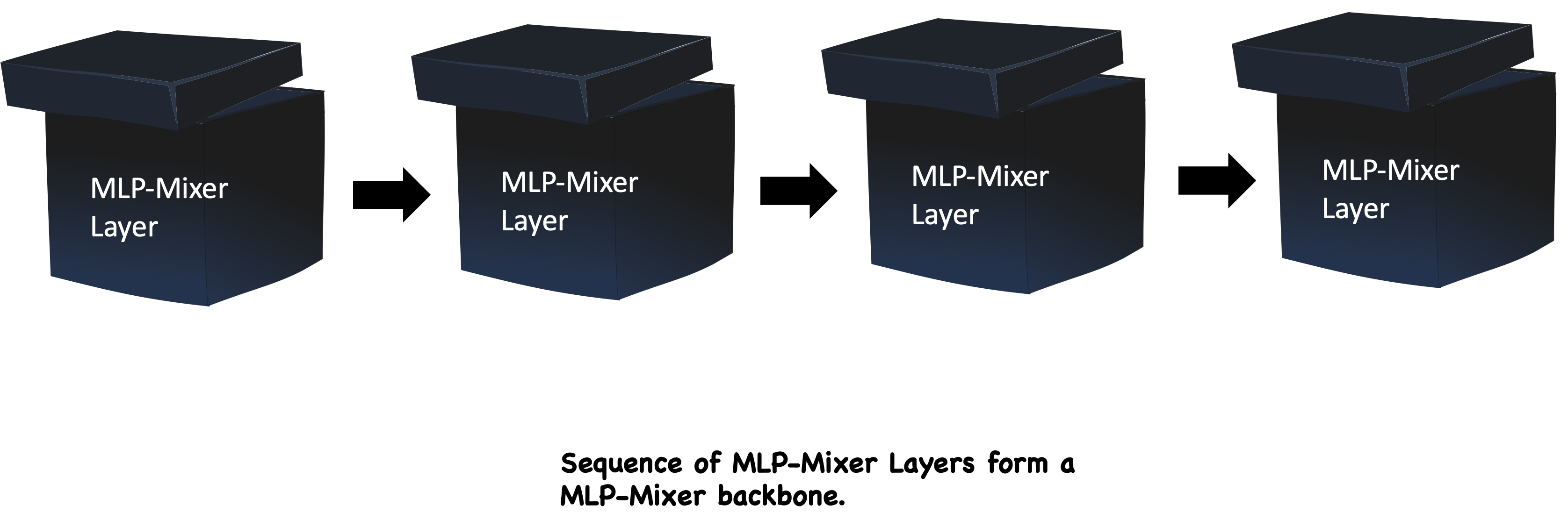
The multi-dimensional tensor is subsequently passed to the PatchTSMixer backbone, which is composed of a sequence of MLP Mixer layers. Each MLP Mixer layer learns inter-patch, intra-patch, and inter-channel correlations through a series of permutation and MLP operations.

PatchTSMixer also employs residual connections and gated attentions to prioritize important features.

Hence, a sequence of MLP Mixer layers creates the following PatchTSMixer backbone.

PatchTSMixer has a modular design to seamlessly support masked time series pretraining as well as direct time series forecasting.

Installation

This demo requires Hugging Face Transformers for the model and the IBM tsfm package for auxiliary data pre-processing. Both can be installed by following the steps below.

1. Install IBM Time Series Foundation Model Repository tsfm.

pip install git+https://github.com/IBM/tsfm.git

2. Install Hugging Face Transformers

pip install transformers

3. Test it with the following commands in a python terminal.

from transformers import PatchTSMixerConfig
from tsfm_public.toolkit.dataset import ForecastDFDataset

Part 1: Forecasting on Electricity dataset

Here we train a PatchTSMixer model directly on the Electricity dataset, and evaluate its performance.

import os
import random

from transformers import (
    EarlyStoppingCallback,
    PatchTSMixerConfig,
    PatchTSMixerForPrediction,
    Trainer,
    TrainingArguments,
)
import numpy as np
import pandas as pd
import torch

from tsfm_public.toolkit.dataset import ForecastDFDataset
from tsfm_public.toolkit.time_series_preprocessor import TimeSeriesPreprocessor
from tsfm_public.toolkit.util import select_by_index

Set seed

from transformers import set_seed

set_seed(42)

Load and prepare datasets

In the next cell, please adjust the following parameters to suit your application:

• dataset_path: path to local .csv file, or web address to a csv file for the data of interest. Data is loaded with pandas, so anything supported by pd.read_csv is supported: (https://pandas.pydata.org/pandas-docs/stable/reference/api/pandas.read_csv.html).
• timestamp_column: column name containing timestamp information, use None if there is no such column.
• id_columns: List of column names specifying the IDs of different time series. If no ID column exists, use [].
• forecast_columns: List of columns to be modeled.
• context_length: The amount of historical data used as input to the model. Windows of the input time series data with length equal to context_length will be extracted from the input dataframe. In the case of a multi-time series dataset, the context windows will be created so that they are contained within a single time series (i.e., a single ID).
• forecast_horizon: Number of timestamps to forecast in the future.
• train_start_index, train_end_index: the start and end indices in the loaded data which delineate the training data.
• valid_start_index, valid_end_index: the start and end indices in the loaded data which delineate the validation data.
• test_start_index, test_end_index: the start and end indices in the loaded data which delineate the test data.
• num_workers: Number of CPU workers in the PyTorch dataloader.
• batch_size: Batch size. The data is first loaded into a Pandas dataframe and split into training, validation, and test parts. Then the Pandas dataframes are converted to the appropriate PyTorch dataset required for training.

# Download ECL data from https://github.com/zhouhaoyi/Informer2020
dataset_path = "~/Downloads/ECL.csv"
timestamp_column = "date"
id_columns = []

context_length = 512
forecast_horizon = 96
num_workers = 16  # Reduce this if you have low number of CPU cores
batch_size = 64  # Adjust according to GPU memory

data = pd.read_csv(
    dataset_path,
    parse_dates=[timestamp_column],
)
forecast_columns = list(data.columns[1:])

# get split
num_train = int(len(data) * 0.7)
num_test = int(len(data) * 0.2)
num_valid = len(data) - num_train - num_test
border1s = [
    0,
    num_train - context_length,
    len(data) - num_test - context_length,
]
border2s = [num_train, num_train + num_valid, len(data)]

train_start_index = border1s[0]  # None indicates beginning of dataset
train_end_index = border2s[0]

# we shift the start of the evaluation period back by context length so that
# the first evaluation timestamp is immediately following the training data
valid_start_index = border1s[1]
valid_end_index = border2s[1]

test_start_index = border1s[2]
test_end_index = border2s[2]

train_data = select_by_index(
    data,
    id_columns=id_columns,
    start_index=train_start_index,
    end_index=train_end_index,
)
valid_data = select_by_index(
    data,
    id_columns=id_columns,
    start_index=valid_start_index,
    end_index=valid_end_index,
)
test_data = select_by_index(
    data,
    id_columns=id_columns,
    start_index=test_start_index,
    end_index=test_end_index,
)

time_series_processor = TimeSeriesPreprocessor(
    context_length=context_length,
    timestamp_column=timestamp_column,
    id_columns=id_columns,
    input_columns=forecast_columns,
    output_columns=forecast_columns,
    scaling=True,
)
time_series_processor.train(train_data)

train_dataset = ForecastDFDataset(
    time_series_processor.preprocess(train_data),
    id_columns=id_columns,
    timestamp_column="date",
    input_columns=forecast_columns,
    output_columns=forecast_columns,
    context_length=context_length,
    prediction_length=forecast_horizon,
)
valid_dataset = ForecastDFDataset(
    time_series_processor.preprocess(valid_data),
    id_columns=id_columns,
    timestamp_column="date",
    input_columns=forecast_columns,
    output_columns=forecast_columns,
    context_length=context_length,
    prediction_length=forecast_horizon,
)
test_dataset = ForecastDFDataset(
    time_series_processor.preprocess(test_data),
    id_columns=id_columns,
    timestamp_column="date",
    input_columns=forecast_columns,
    output_columns=forecast_columns,
    context_length=context_length,
    prediction_length=forecast_horizon,
)

Configure the PatchTSMixer model

Next, we instantiate a randomly initialized PatchTSMixer model with a configuration. The settings below control the different hyperparameters related to the architecture.

• num_input_channels: the number of input channels (or dimensions) in the time series data. This is automatically set to the number for forecast columns.
• context_length: As described above, the amount of historical data used as input to the model.
• prediction_length: This is same as the forecast horizon as described above.
• patch_length: The patch length for the PatchTSMixer model. It is recommended to choose a value that evenly divides context_length.
• patch_stride: The stride used when extracting patches from the context window.
• d_model: Hidden feature dimension of the model.
• num_layers: The number of model layers.
• dropout: Dropout probability for all fully connected layers in the encoder.
• head_dropout: Dropout probability used in the head of the model.
• mode: PatchTSMixer operating mode. "common_channel"/"mix_channel". Common-channel works in channel-independent mode. For pretraining, use "common_channel".
• scaling: Per-widow standard scaling. Recommended value: "std".

For full details on the parameters, we refer to the documentation.

We recommend that you only adjust the values in the next cell.

patch_length = 8
config = PatchTSMixerConfig(
    context_length=context_length,
    prediction_length=forecast_horizon,
    patch_length=patch_length,
    num_input_channels=len(forecast_columns),
    patch_stride=patch_length,
    d_model=16,
    num_layers=8,
    expansion_factor=2,
    dropout=0.2,
    head_dropout=0.2,
    mode="common_channel",
    scaling="std",
)
model = PatchTSMixerForPrediction(config)

Train model

Next, we can leverage the Hugging Face Trainer class to train the model based on the direct forecasting strategy. We first define the TrainingArguments which lists various hyperparameters regarding training such as the number of epochs, learning rate, and so on.

training_args = TrainingArguments(
    output_dir="./checkpoint/patchtsmixer/electricity/pretrain/output/",
    overwrite_output_dir=True,
    learning_rate=0.001,
    num_train_epochs=100,  # For a quick test of this notebook, set it to 1
    do_eval=True,
    evaluation_strategy="epoch",
    per_device_train_batch_size=batch_size,
    per_device_eval_batch_size=batch_size,
    dataloader_num_workers=num_workers,
    report_to="tensorboard",
    save_strategy="epoch",
    logging_strategy="epoch",
    save_total_limit=3,
    logging_dir="./checkpoint/patchtsmixer/electricity/pretrain/logs/",  # Make sure to specify a logging directory
    load_best_model_at_end=True,  # Load the best model when training ends
    metric_for_best_model="eval_loss",  # Metric to monitor for early stopping
    greater_is_better=False,  # For loss
    label_names=["future_values"],
)

# Create the early stopping callback
early_stopping_callback = EarlyStoppingCallback(
    early_stopping_patience=10,  # Number of epochs with no improvement after which to stop
    early_stopping_threshold=0.0001,  # Minimum improvement required to consider as improvement
)

# define trainer
trainer = Trainer(
    model=model,
    args=training_args,
    train_dataset=train_dataset,
    eval_dataset=valid_dataset,
    callbacks=[early_stopping_callback],
)

# pretrain
trainer.train()

>>> | Epoch | Training Loss | Validation Loss |
    |-------|---------------|------------------|
    |   1   |    0.247100   |     0.141067     |
    |   2   |    0.168600   |     0.127757     |
    |   3   |    0.156500   |     0.122327     |
    ...

Evaluate the model on the test set

Note that the training and evaluation loss for PatchTSMixer is the Mean Squared Error (MSE) loss. Hence, we do not separately compute the MSE metric in any of the following evaluation experiments.

results = trainer.evaluate(test_dataset)
print("Test result:")
print(results)

>>> Test result:
    {'eval_loss': 0.12884521484375, 'eval_runtime': 5.7532, 'eval_samples_per_second': 897.763, 'eval_steps_per_second': 3.65, 'epoch': 35.0}

We get an MSE score of 0.128 which is the SOTA result on the Electricity data.

Save model

save_dir = "patchtsmixer/electricity/model/pretrain/"
os.makedirs(save_dir, exist_ok=True)
trainer.save_model(save_dir)

Part 2: Transfer Learning from Electricity to ETTh2

In this section, we will demonstrate the transfer learning capability of the PatchTSMixer model. We use the model pre-trained on the Electricity dataset to do zero-shot forecasting on the ETTh2 dataset.

By Transfer Learning, we mean that we first pretrain the model for a forecasting task on a source dataset (which we did above on the Electricity dataset). Then, we will use the pretrained model for zero-shot forecasting on a target dataset. By zero-shot, we mean that we test the performance in the target domain without any additional training. We hope that the model gained enough knowledge from pretraining which can be transferred to a different dataset.

Subsequently, we will do linear probing and (then) finetuning of the pretrained model on the train split of the target data, and will validate the forecasting performance on the test split of the target data. In this example, the source dataset is the Electricity dataset and the target dataset is ETTh2.

Transfer Learning on ETTh2 data

All evaluations are on the test part of the ETTh2 data: Step 1: Directly evaluate the electricity-pretrained model. This is the zero-shot performance.
Step 2: Evalute after doing linear probing.
Step 3: Evaluate after doing full finetuning.

Load ETTh2 dataset

Below, we load the ETTh2 dataset as a Pandas dataframe. Next, we create 3 splits for training, validation and testing. We then leverage the TimeSeriesPreprocessor class to prepare each split for the model.

dataset = "ETTh2"

dataset_path = f"https://raw.githubusercontent.com/zhouhaoyi/ETDataset/main/ETT-small/{dataset}.csv"
timestamp_column = "date"
id_columns = []
forecast_columns = ["HUFL", "HULL", "MUFL", "MULL", "LUFL", "LULL", "OT"]
train_start_index = None  # None indicates beginning of dataset
train_end_index = 12 * 30 * 24

# we shift the start of the evaluation period back by context length so that
# the first evaluation timestamp is immediately following the training data
valid_start_index = 12 * 30 * 24 - context_length
valid_end_index = 12 * 30 * 24 + 4 * 30 * 24

test_start_index = 12 * 30 * 24 + 4 * 30 * 24 - context_length
test_end_index = 12 * 30 * 24 + 8 * 30 * 24

data = pd.read_csv(
    dataset_path,
    parse_dates=[timestamp_column],
)

train_data = select_by_index(
    data,
    id_columns=id_columns,
    start_index=train_start_index,
    end_index=train_end_index,
)
valid_data = select_by_index(
    data,
    id_columns=id_columns,
    start_index=valid_start_index,
    end_index=valid_end_index,
)
test_data = select_by_index(
    data,
    id_columns=id_columns,
    start_index=test_start_index,
    end_index=test_end_index,
)

time_series_processor = TimeSeriesPreprocessor(
    context_length=context_length
    timestamp_column=timestamp_column,
    id_columns=id_columns,
    input_columns=forecast_columns,
    output_columns=forecast_columns,
    scaling=True,
)
time_series_processor.train(train_data)

>>> TimeSeriesPreprocessor {
        "context_length": 512,
        "feature_extractor_type": "TimeSeriesPreprocessor",
        "id_columns": [],
    ...
    }

train_dataset = ForecastDFDataset(
    time_series_processor.preprocess(train_data),
    id_columns=id_columns,
    input_columns=forecast_columns,
    output_columns=forecast_columns,
    context_length=context_length,
    prediction_length=forecast_horizon,
)
valid_dataset = ForecastDFDataset(
    time_series_processor.preprocess(valid_data),
    id_columns=id_columns,
    input_columns=forecast_columns,
    output_columns=forecast_columns,
    context_length=context_length,
    prediction_length=forecast_horizon,
)
test_dataset = ForecastDFDataset(
    time_series_processor.preprocess(test_data),
    id_columns=id_columns,
    input_columns=forecast_columns,
    output_columns=forecast_columns,
    context_length=context_length,
    prediction_length=forecast_horizon,
)

Zero-shot forecasting on ETTh2

As we are going to test forecasting performance out-of-the-box, we load the model which we pretrained above.

from transformers import PatchTSMixerForPrediction

finetune_forecast_model = PatchTSMixerForPrediction.from_pretrained(
    "patchtsmixer/electricity/model/pretrain/"
)

finetune_forecast_args = TrainingArguments(
    output_dir="./checkpoint/patchtsmixer/transfer/finetune/output/",
    overwrite_output_dir=True,
    learning_rate=0.0001,
    num_train_epochs=100,
    do_eval=True,
    evaluation_strategy="epoch",
    per_device_train_batch_size=batch_size,
    per_device_eval_batch_size=batch_size,
    dataloader_num_workers=num_workers,
    report_to="tensorboard",
    save_strategy="epoch",
    logging_strategy="epoch",
    save_total_limit=3,
    logging_dir="./checkpoint/patchtsmixer/transfer/finetune/logs/",  # Make sure to specify a logging directory
    load_best_model_at_end=True,  # Load the best model when training ends
    metric_for_best_model="eval_loss",  # Metric to monitor for early stopping
    greater_is_better=False,  # For loss
)

# Create a new early stopping callback with faster convergence properties
early_stopping_callback = EarlyStoppingCallback(
    early_stopping_patience=5,  # Number of epochs with no improvement after which to stop
    early_stopping_threshold=0.001,  # Minimum improvement required to consider as improvement
)

finetune_forecast_trainer = Trainer(
    model=finetune_forecast_model,
    args=finetune_forecast_args,
    train_dataset=train_dataset,
    eval_dataset=valid_dataset,
    callbacks=[early_stopping_callback],
)

print("\n\nDoing zero-shot forecasting on target data")
result = finetune_forecast_trainer.evaluate(test_dataset)
print("Target data zero-shot forecasting result:")
print(result)

>>> Doing zero-shot forecasting on target data

    Target data zero-shot forecasting result:
    {'eval_loss': 0.3038313388824463, 'eval_runtime': 1.8364, 'eval_samples_per_second': 1516.562, 'eval_steps_per_second': 5.99}

As can be seen, we get a mean-squared error (MSE) of 0.3 zero-shot which is near to the state-of-the-art result.

Next, let's see how we can do by performing linear probing, which involves training a linear classifier on top of a frozen pre-trained model. Linear probing is often done to test the performance of features of a pretrained model.

Linear probing on ETTh2

We can do a quick linear probing on the train part of the target data to see any possible test performance improvement.

# Freeze the backbone of the model
for param in finetune_forecast_trainer.model.model.parameters():
    param.requires_grad = False

print("\n\nLinear probing on the target data")
finetune_forecast_trainer.train()
print("Evaluating")
result = finetune_forecast_trainer.evaluate(test_dataset)
print("Target data head/linear probing result:")
print(result)
    
>>> Linear probing on the target data


    | Epoch | Training Loss | Validation Loss |
    |-------|---------------|------------------|
    |   1   |    0.447000   |     0.216436     |
    |   2   |    0.438600   |     0.215667     |
    |   3   |    0.429400   |     0.215104     |
    ...

    Evaluating

    Target data head/linear probing result:
    {'eval_loss': 0.27119266986846924, 'eval_runtime': 1.7621, 'eval_samples_per_second': 1580.478, 'eval_steps_per_second': 6.242, 'epoch': 13.0}

As can be seen, by training a simple linear layer on top of the frozen backbone, the MSE decreased from 0.3 to 0.271 achieving state-of-the-art results.

save_dir = f"patchtsmixer/electricity/model/transfer/{dataset}/model/linear_probe/"
os.makedirs(save_dir, exist_ok=True)
finetune_forecast_trainer.save_model(save_dir)

save_dir = f"patchtsmixer/electricity/model/transfer/{dataset}/preprocessor/"
os.makedirs(save_dir, exist_ok=True)
time_series_processor.save_pretrained(save_dir)

>>> ['patchtsmixer/electricity/model/transfer/ETTh2/preprocessor/preprocessor_config.json']

Finally, let's see if we get any more improvements by doing a full finetune of the model on the target dataset.

Full finetuning on ETTh2

We can do a full model finetune (instead of probing the last linear layer as shown above) on the train part of the target data to see a possible test performance improvement. The code looks similar to the linear probing task above, except that we are not freezing any parameters.

# Reload the model
finetune_forecast_model = PatchTSMixerForPrediction.from_pretrained(
    "patchtsmixer/electricity/model/pretrain/"
)
finetune_forecast_trainer = Trainer(
    model=finetune_forecast_model,
    args=finetune_forecast_args,
    train_dataset=train_dataset,
    eval_dataset=valid_dataset,
    callbacks=[early_stopping_callback],
)
print("\n\nFinetuning on the target data")
finetune_forecast_trainer.train()
print("Evaluating")
result = finetune_forecast_trainer.evaluate(test_dataset)
print("Target data full finetune result:")
print(result)

>>> Finetuning on the target data

    | Epoch | Training Loss | Validation Loss |
    |-------|---------------|-----------------|
    |   1   |    0.432900   |     0.215200    |
    |   2   |    0.416700   |     0.210919    |
    |   3   |    0.401400   |     0.209932    |
    ...

    Evaluating

    Target data full finetune result:
    {'eval_loss': 0.2734043300151825, 'eval_runtime': 1.5853, 'eval_samples_per_second': 1756.725, 'eval_steps_per_second': 6.939, 'epoch': 9.0}

In this case, there is not much improvement by doing full finetuning. Let's save the model anyway.

save_dir = f"patchtsmixer/electricity/model/transfer/{dataset}/model/fine_tuning/"
os.makedirs(save_dir, exist_ok=True)
finetune_forecast_trainer.save_model(save_dir)

Summary

In this blog, we presented a step-by-step guide on leveraging PatchTSMixer for tasks related to forecasting and transfer learning. We intend to facilitate the seamless integration of the PatchTSMixer HF model for your forecasting use cases. We trust that this content serves as a useful resource to expedite your adoption of PatchTSMixer. Thank you for tuning in to our blog, and we hope you find this information beneficial for your projects.