I explored several optical illusions and “trompe l’oeil” post-processing effects in Post-Processing Shaders as a Creative Medium that create the illusion of texture or material, like woven crochet or glass. Halftone is, funnily enough, not so different as it is inherently an optical illusion itself.

The effect creates the impression of continuous/smooth tones, much like dithering, by providing a high-frequency grid of dots. Because these dots can be smaller than the eye's spatial resolution, the brain ends up performing a spatial average of the pattern. Thus, past a certain dot radius, we stop seeing individual dots composing the grid and instead see the ratio of 'ink' to 'empty space' as smooth tones.

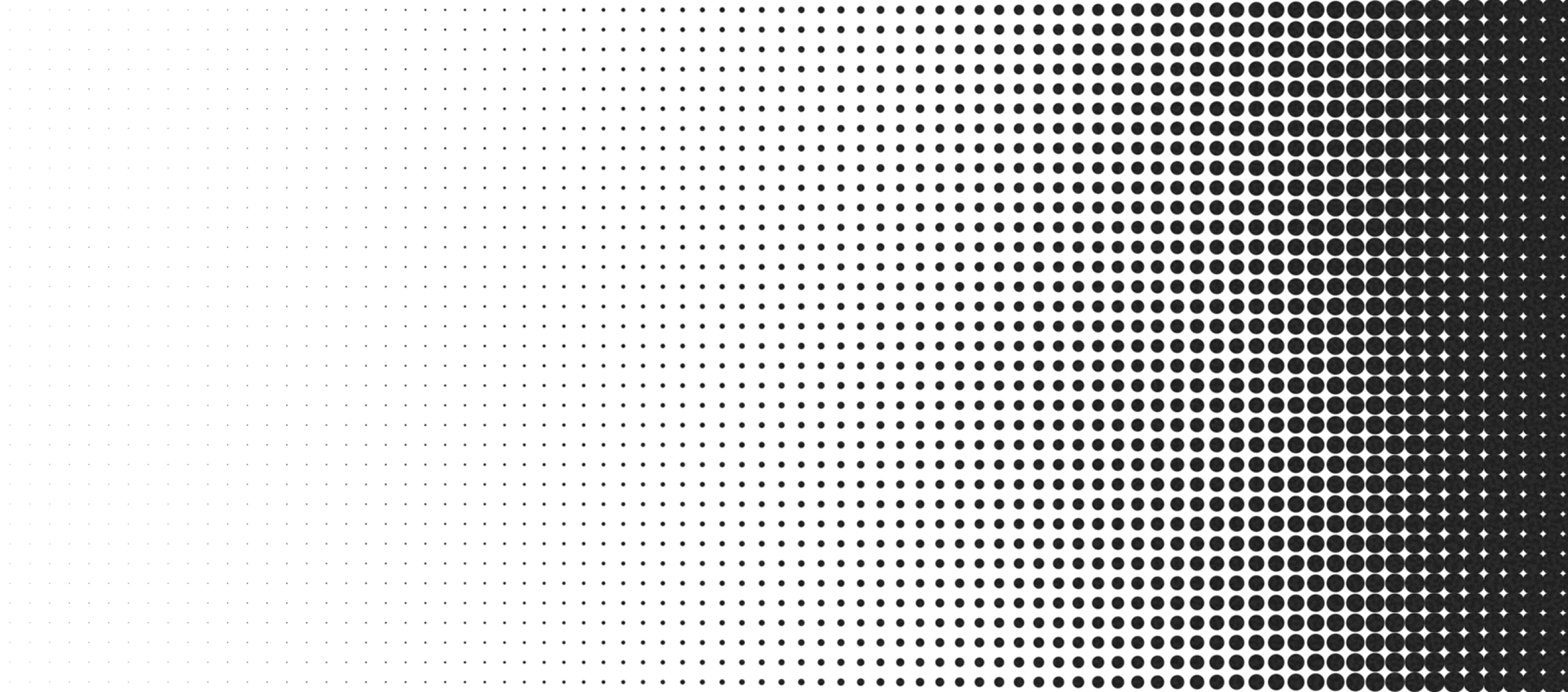
We will use those characteristics to guide and break down our implementation of halftone as a shader with GLSL.

Rendering a grid of dots

To ensure this article is as approachable as possible to beginners, we’re going to build this effect from the ground up, starting with its most fundamental pieces. The first step is, as you may expect, to render a single dot or circle using GLSL and UV coordinates.

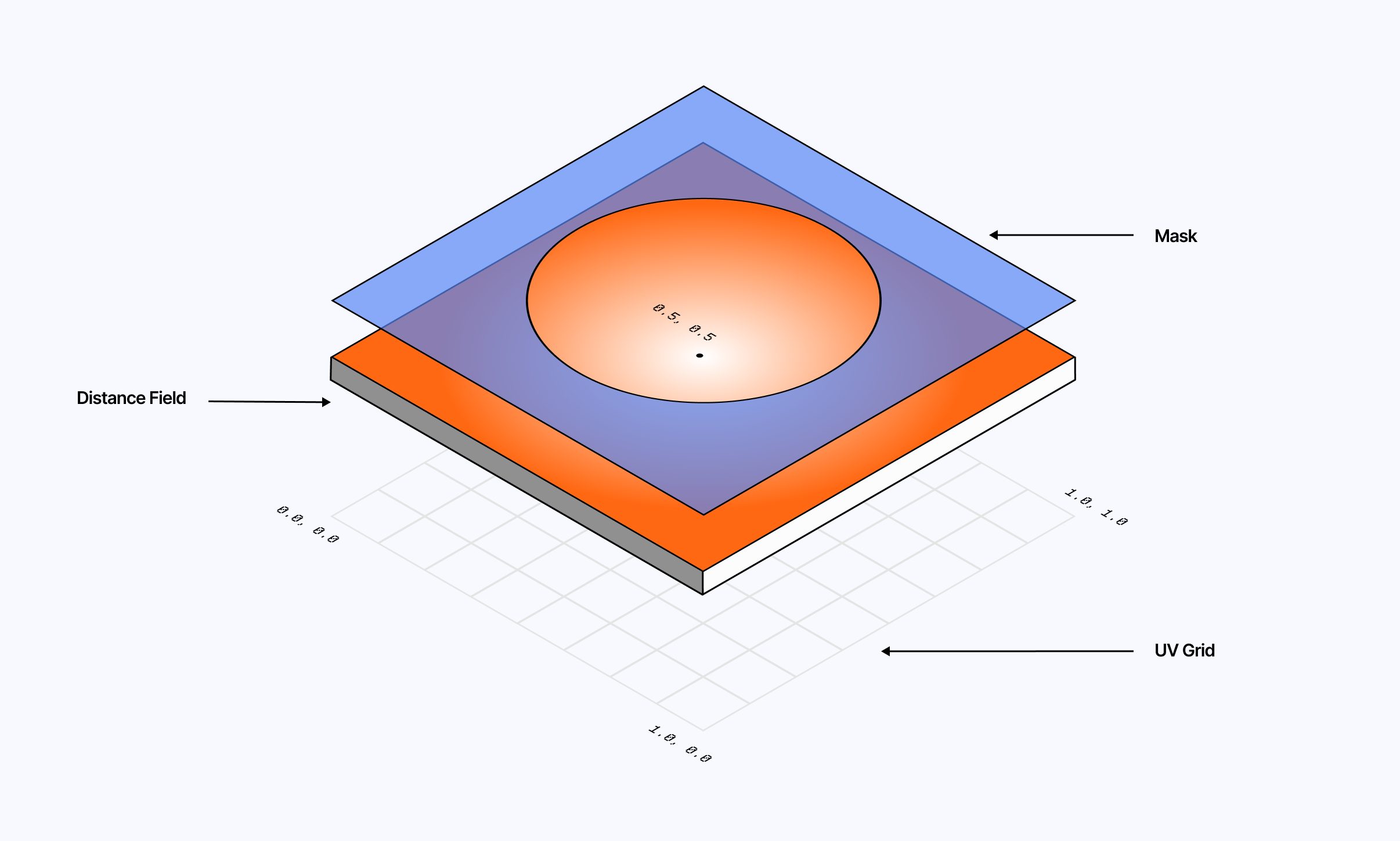
The diagram above illustrates the two key aspects of drawing a circle in a fragment shader:

1. A distance d that represents the distance to the center point {0.5, 0.5} of our UV coordinate system. The results this yield is also called a distance field

2. A mask: a threshold from which we decide what is in the dot, and what is outside.

1
float dist = length(cellUv - 0.5);
2
float circle = step(0.35, dist);
4
vec3 color = mix(vec3(1.0), vec3(0.0), circle);

By adjusting the mask function, we can also choose whether we prefer a softer or more defined result.

1
float dist = length(cellUv - 0.5);
2
float circle = smoothstep(0.32, 0.37, dist);
4
vec3 color = mix(vec3(1.0), vec3(0.0), circle);

With that, we now have the fundamental shape for our halftone effect and can focus on its second main characteristic, the grid. In GLSL, a grid can be achieved via the fract ¹ function, which returns the fractional part of its number argument:

• fract(1.1) returns 0.1

• fract(0.9) returns 0.9

• fract(20.3) returns 0.3

Essentially, it is equivalent to doing mod(x, 1), which returns any number after the floating point of x. Of course, if we just do fract(uv), nothing will change, since our UVs are already defined within the standard 0.0 → 1.0 range. What we need to do first is scale our UV coordinates by multiplying them by our grid size, and then use the scaled UVs as an argument for fract, which will result in our fragment shader tiling. The diagram below showcases our UV coordinates before and after tiling.

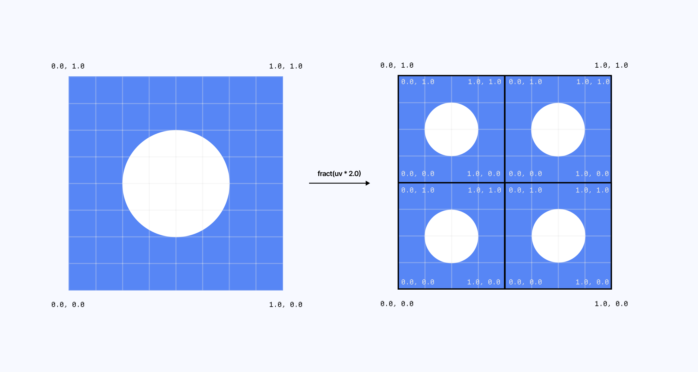
Notice how we now have multiple cells, each with their own UV coordinates ranging from 0.0 -> 1.0 and essentially running the same fragment shader. If we combine this with our circle code from above, each of these cell will draw its own circle, thus giving us our grid of dots!

The widget below showcases that and lets you:

• Scale up and down the grid.

• Scale up and down the scale of the radius.

while also displaying some variation in dot size, so you can start seeing the halftone effect at play with this very simple example.

5
uniform vec2 uResolution;
7
uniform float uGridSize;
10
  vec2 cellUv = fract(vUv * uGridSize);
12
  float dist = length(cellUv - 0.5);
13
  float radius = uRadius * max(max(vUv.x, vUv.y), 0.2);
15
  float circle = smoothstep(radius - 0.01, radius + 0.01, dist);
16
  vec3 color = mix(vec3(0.4, 0.75, 1.0), vec3(0.0, 0.0, 0.0), circle);
17
  fragColor = vec4(color, 1.0);

Applying Halftone

While playing with dot radii can yield some beautiful patterns, one of the main appeals of halftone is to apply it as a filter on top of a 3D scene, image, or video. The result comes with a loss of details from the underlying media, but what we obtain in return is a kind of microtexture that fills in empty spaces with interesting shapes where we’d normally see flat colors.

If we simply apply the grid of dots from the previous section as a filter and color the dots based on the sampled pixels at that position, we’re only going to see a simple mask. To achieve a true halftone effect, we need to process our underlying texture first by pixelating it in such a way that it matches 1:1 our grid of dots.

An interesting aspect of this pixelization logic is how we rely on the floor function to define our pixelatedUV coordinates. This function removes the decimals of our UV coordinates, the opposite effect of fract, and thus ensures that each pixel within a given cell samples the same color, thus resulting in a pixelated look and feel for our texture.

2
vec2 normalizedPixelSize = uPixelSize / uResolution;
3
vec2 uvPixel = normalizedPixelSize * floor(uv / normalizedPixelSize);
5
vec4 color = texture(inputBuffer, uvPixel);
7
vec2 cellUv = fract(uv / normalizedPixelSize);
8
float dist = length(cellUv - 0.5);
10
float circle = smoothstep(uRadius - 0.01, uRadius + 0.01, dist);
12
color = mix(color, vec4(0.0, 0.0, 0.0, 1.0), circle);

Combining this with our grid of dots, like in the code snippet above, brings us one step closer to a halftone effect.

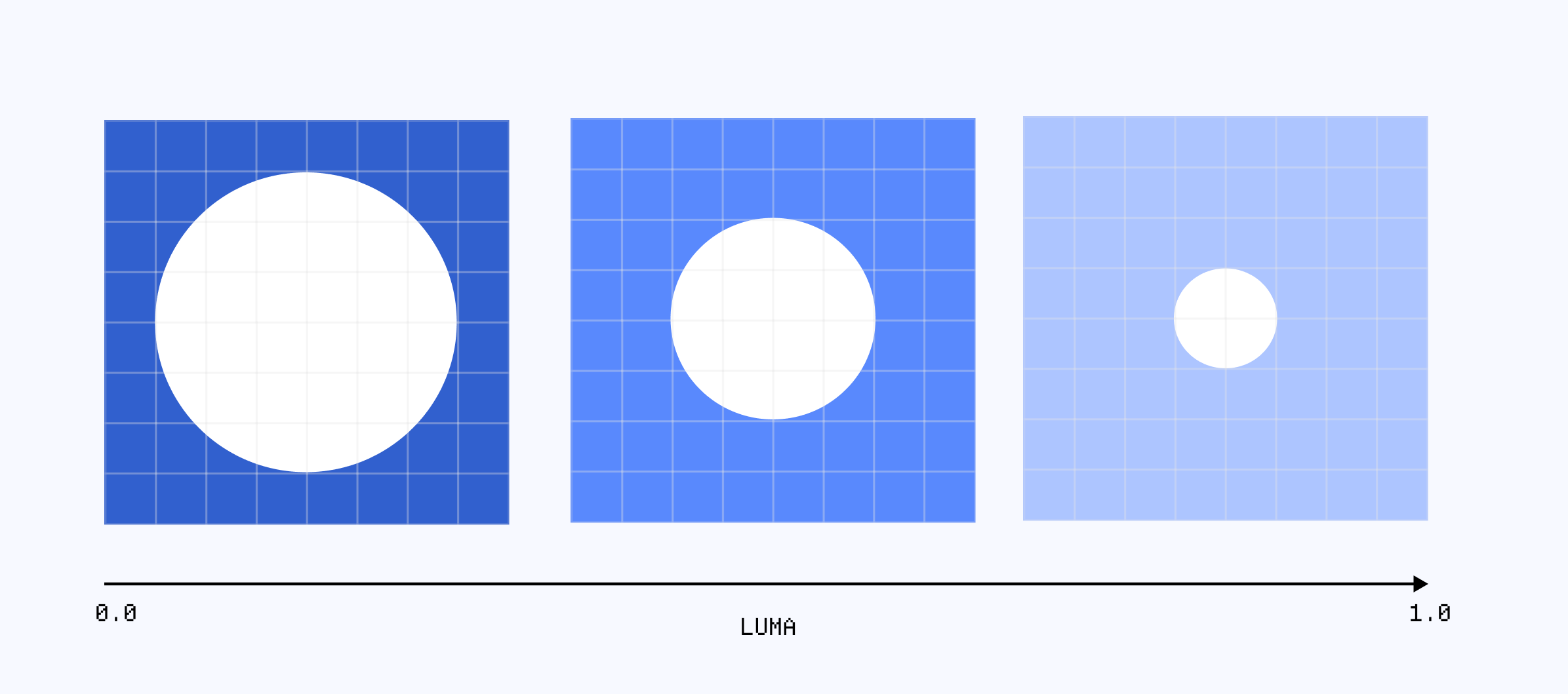
Of course, there’s still something missing here from our original definition of halftone, the variation of dot size! We can implement this easily by using the luma of a given pixel, and tweak the radius based on its value.

2
vec2 normalizedPixelSize = uPixelSize / uResolution;
3
vec2 uvPixel = normalizedPixelSize * floor(uv / normalizedPixelSize);
5
vec4 color = texture(inputBuffer, uvPixel);
6
float luma = dot(vec3(0.2126, 0.7152, 0.0722), color.rgb);
7
float radius = uRadius * (0.1 + luma);
9
vec2 cellUv = fract(uv / normalizedPixelSize);
10
float dist = length(cellUv - 0.5);
12
float circle = smoothstep(radius - 0.01, radius + 0.01, dist);
14
color = mix(color, vec4(0.0, 0.0, 0.0, 1.0), circle);

Moreover, if we wanted to display a grayscale version of our halftone, we could also do so using that same value, which you can see the result below by toggling on the "Luma-based radius" and changing the color mode of the output.

More interesting variants of halftone can be achieved by introducing a grid offset, thus staggering the dots instead of having them perfectly aligned. This allows for a higher density of dots in our pattern, reducing the amount of white space. This offset is defined by tweaking our UVs, thus propagating it not only in how we lay down our dots but also how we sample our texture and pixelize it.

2
vec2 normalizedPixelSize = pixelSize / resolution;
5
float rowIndex = floor(uv.y / normalizedPixelSize.y);
6
if (offset && mod(rowIndex, 2.0) == 1.0) {
7
    offsetUv.x += normalizedPixelSize.x * 0.5;
10
vec2 uvPixel = normalizedPixelSize * floor(offsetUv / normalizedPixelSize);
11
vec4 color = texture2D(inputBuffer, uvPixel);

The playground below implements this on top of a React Three Fiber 3D scene, thus letting you not only explore this variant alongside all the others we’ve seen so far but also play with many of the settings over a dynamic scene where I think halftone shines the most: on top of organic-moving objects, bringing a lovely contrasting aesthetic to the scene.

Not just dots

When the Paper team announced their halftone presets, back in November 2025, they showcased a lot of halftone variants I had not seen before. It turns out that circles are just a part of the wide spectrum of halftone patterns available, and we can allow ourselves to tweak the original definition of the effect with what I dubbed “dot adjacent” shapes.

The first one we can take a look at is directly inspired by the video featured in the tweet above: dots and squares, which is a combination of:

• The classic dot pattern we implemented already

• An inverted pattern where we can find white dots inside colored pixels. The darker the underlying pixel, the bigger the white dot.

Those two patterns complement each other very well, and can be mixed and matched based on luma, as showcased in the demo below:

• A darker pixel would yield a “square with white dot.”

• A lighter pixel would yield a standard dot.

This has the effect of preserving much more of the original texture while still making the brighter parts of it standard halftone.

We can also choose to go all in one of the patterns as showcased below, where I overlaid the different patterns on top of a video so we can see the effect at play on a subtly dynamic media:

Another type of halftone I found interesting to highlight is the ring variant. I originally got inspired some of the work of @poetengineer__ who made some beautiful uncommon halftone renders:

Making a ring is actually simpler than it looks: we just need to define two circles, and combine them using an A AND NOT B combinatory logic.

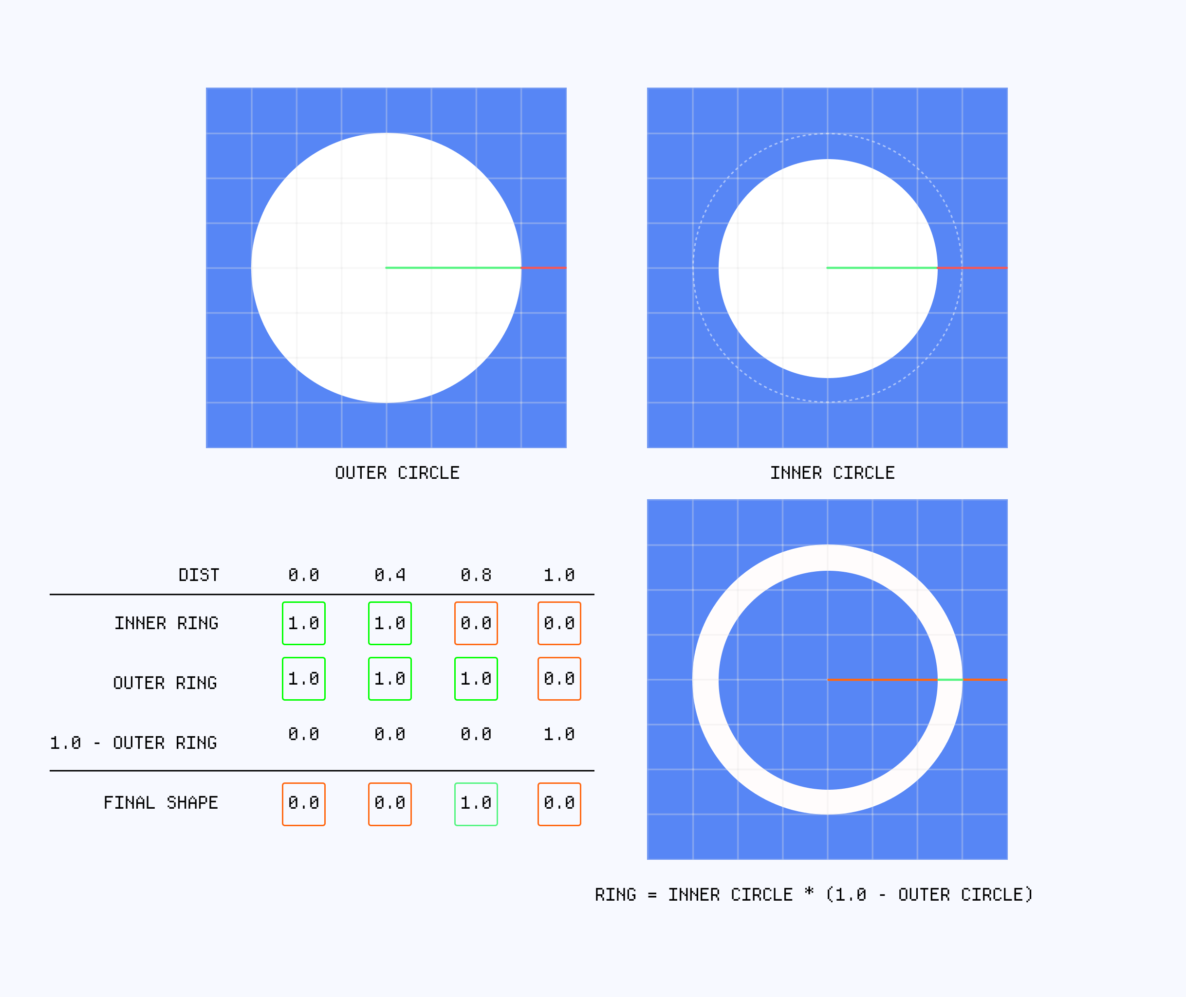
3
float radius = uRadius * (0.2 + luma);
5
float ringThickness = 0.1;
6
float innerRadius = radius - ringThickness;
8
float outerCircle = smoothstep(radius - 0.01, radius + 0.01, dist);
9
float innerCircle = smoothstep(innerRadius - 0.01, innerRadius + 0.01, dist);
11
float ring = innerCircle * (1.0 - outerCircle);
13
color = mix(vec4(0.0, 0.0, 0.0, 1.0), color, ring);

Applying this effect with a monochromatic palette to a video yields a technical/low-res aesthetic, almost terminal-like, unlike the more in-your-face and high contrast big bright dots of your standard halftone variant.

Until now, we have considered the case of a monochromatic halftone, where the tones are defined by the concentration of dots in a single grid. We also tried our hand at “colored” halftone, but we were merely picking up colors from the underlying texture/media and not really pushing the optical illusion of this effect to its full extent.

Indeed, instead of treating halftone as a simple grid, we can also view it as a stack of grids, where each layer corresponds to a specific color channel of the underlying image. We can derive our layers defined through the Red, Green, and Blue color channels for an RGB look, or Cyan, Magenta, Yellow, and Key for a classic CMYK printing finish. This technique will expand what we can do with regard to building halftone shaders, but it will also come at a cost of visual artifacts and interference, which we must first understand to work around them.

Moiré Pattern

You may have encountered Moiré patterns in your renders from time to time when experimenting with overlapping repeating patterns. This type of interference manifests when two almost identical patterns are overlaid on top of each other ³. By almost identical, here I mean:

• They could not be completely identical, for example, different frequencies.

• They could be identical, but need to be displaced or rotated.

It occurs in both physical and digital media alike, and is yet another optical illusion / perception artifact due to our brain trying to reconcile the intersection of two competing patterns.

The widget below demonstrates this effect on very simple examples for you to try:

• We have a version where two grids are stacked on top of each other. Rotating one will cause quite a few interferences.

• The other example consists of a two stacked Poisson distribution, where the slightest rotation reveals circular interferences.

The GLSL implementation is rather straightforward and can serve you as a base for your own Moiré-like experiences.

1
mat2 rotate(float angle) {
4
  return mat2(c, -s, s, c);
7
float circleGrid(vec2 uv, float radius, float angle) {
8
  vec2 normalizedPixelSize = uPixelSize / uResolution;
11
  vec2 uvPx = uv * uResolution;
12
  vec2 rotatedPx = rotate(angle) * uvPx;
13
  vec2 rotatedUv = rotatedPx / uResolution;
15
  vec2 cellUv = fract(rotatedUv / normalizedPixelSize);
16
  float dist = length(cellUv - 0.5);
18
  float edgeWidth = fwidth(dist);
20
  float circle = smoothstep(radius - edgeWidth, radius + edgeWidth, dist);
28
  float circleGridA = circleGrid(uv, uRadius, 0.0)
29
  float circleGridB = circleGrid(uv, uRadius, radians(uAngle))
31
  vec3 colorA = mix(vec3(1.0), vec3(0.0), circleGridA);
32
  vec3 colorB = mix(vec3(1.0), vec3(0.0), circleGridB);
34
  fragColor = vec4(max(colorA, colorB), 1.0);

This will inevitably occur in the examples of this section of the article, as we will start building multichannel halftoning. The artifact can be embraced or seen as an issue to mitigate, as the printing industry often does by applying workarounds. In our case, we'll solve this problem by applying specific rotations to each individual layer, thus reducing the interference to a minimum. We will see this technique in action in our upcoming implementation of CMYK halftone.

Digital vs Physical color blending

The main use case for our multichannel implementation of halftone is for each layer to hold a specific color channel and blend into one another, reproducing the optical mixing found in physical print. We can opt for layers representing either:

• RGB for a more digital-like render.

• CMYK for a more physical look.

However, the blending of these two color models differs:

• The former one is based on the addition of light starting from a black display. The red, blue, and green color channels add up to white.

• The latter, on the subtraction of color from light being absorbed, starting from a white paper. The cyan, magenta, and yellow “inks” filter the light hitting them. The more of them overlap, the darker the resulting tone as light gets further filtered, eventually reaching black.

We can see this firsthand below, where I reproduce the RGB and CMY color blending variants on HTML canvases.

Mathematically speaking, here is what is happening. For the RGB variant, we’re simply adding the color intensity of each channel, i.e., ColorOut = (Ir, 0, 0) + (0, Ig, 0) + (0, 0, Ib). Adding/composing color channels is something we do quite often in GLSL for several effects like refraction, or dispersion. As the values approach 1.0, their combination tends towards (1.0, 1.0, 1.0), i.e., white, which is represented in the chart below:

For CMY subtractive blending, which mathematically is a bit of a misnomer, it can be represented through a multiplication: ColorOut = White * (1.0 - C) * (1.0 - M) * (1.0 - Y). The subtractive nature of this blending refers to the physics of light absorption: each color channel acts as a filter that absorbs specific wavelengths from white light, only to leave the leftovers to the viewer. That’s why overlapping all the color channels results in black.

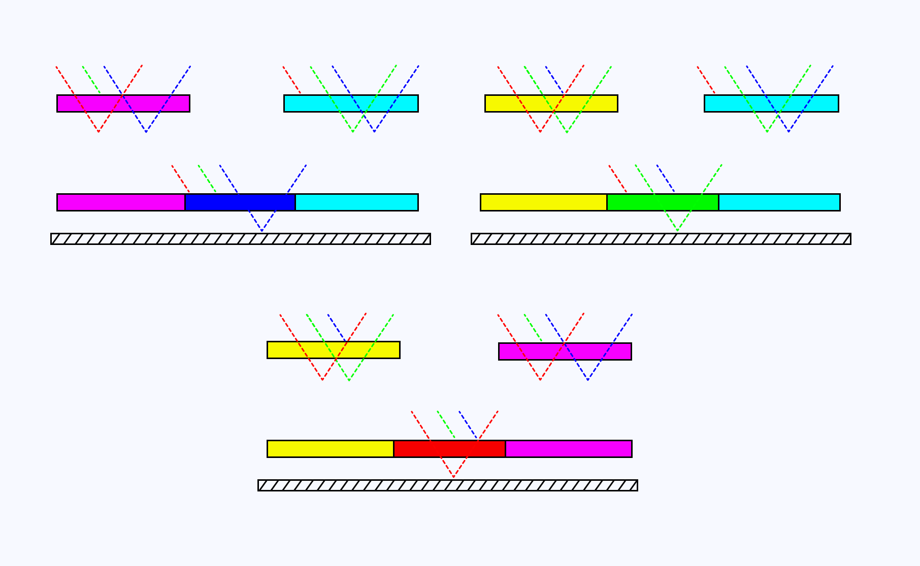
The chart below represents the reflectance profile of cyan, magenta, and yellow across the visible spectrum, as well as the resulting filter:

Notice how the resulting color for the blending corresponds to the overlapping area shared by all the curves.

CMYK halftone

The halftone variant we’re about to look at is perhaps the main reason I wrote the article in the first place. I originally got inspired by some of the work of @floguo who produced some renders where this pattern really shone.

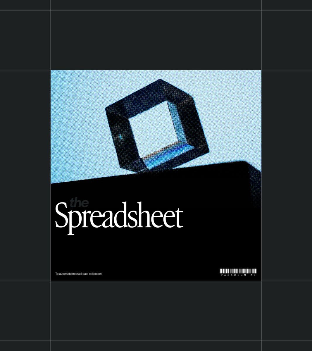
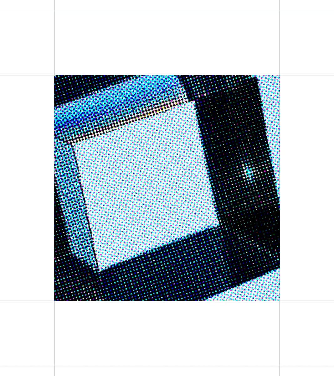
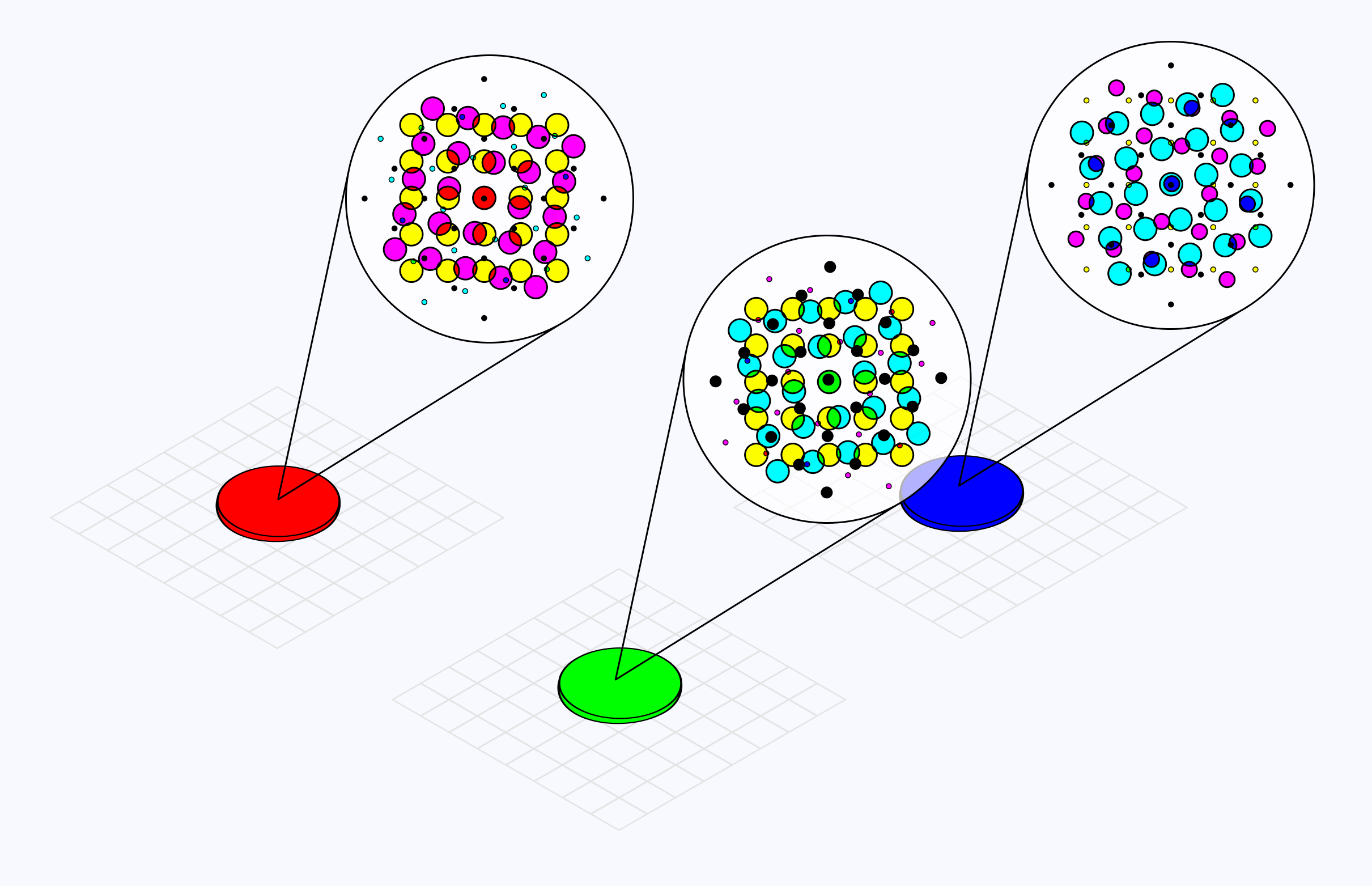
This intrigued me, so I tried my hand at reproducing a shader for it, which nerd-snipped me and led me to learn a lot about color blending, Moiré, and halftone in general. Since, to build this effect, we’d need to overlay 4 distinct grids of dots, doing so naively would immediately give us some Moiré patters and make the colors a bit washed out. Instead, we need to rotate each layer at a specific angle set of angles to yield an image with as few artifacts as possible. The widget below reproduces the CMYK halftone variant with preset angle values of:

• 15.0 for cyan

• 75.0 for magenta

• 0.0 for yellow

• 45.0 for key

I recommend playing with the angle values and dot density to see the differences in output.

As you can see above, the size of the individual dots varies based on the underlying sampled color. With just these 4 colors and the ability to tweak each dots size and density, we can obtain any type of shade necessary to render a colored output, just like print!

Implementation-wise, we can work on top of our classic halftone base. However, we’d first need to convert our sampled color from RGB to CMYK. I used a function from Matt DesLauriers to do so:

1
vec4 RGBtoCMYK (vec3 rgb) {
5
  float k = min(1.0 - r, min(1.0 - g, 1.0 - b));
11
    cmy.x = (1.0 - r - k) / invK;
12
    cmy.y = (1.0 - g - k) / invK;
13
    cmy.z = (1.0 - b - k) / invK;
16
  return clamp(vec4(cmy, k), 0.0, 1.0);

Then, we can generate our grid of dots for each individual channel, and have the coverage/radius of their dots match the intensity of that color channel at that given position on screen.

1
vec2 toGridUV(vec2 uv, float angleDeg) {
2
  return rot(angleDeg) * (uv * resolution) / pixelSize;
5
vec2 getCellCenterUV(vec2 uv, float angleDeg) {
6
  vec2 gridUV = toGridUV(uv, angleDeg);
7
  vec2 cellCenter = floor(gridUV) + 0.5;
8
  vec2 centerScreen = rot(-angleDeg) * cellCenter * pixelSize;
9
  return centerScreen / resolution;
12
float halftoneDot(vec2 uv, float angleDeg, float coverage) {
13
  vec2 gridUV = toGridUV(uv, angleDeg);
14
  vec2 distToCenter = fract(gridUV) - 0.5;
16
  float r = dotSize * sqrt(clamp(coverage, 0.0, 1.0));
17
  float aa = fwidth(length(distToCenter));
18
  float d = length(distToCenter);
19
  return 1.0 - smoothstep(r - aa, r + aa, d);
22
void mainImage(const in vec4 inputColor, const in vec2 uv, out vec4 outputColor) {
23
  vec2 uvC = getCellCenterUV(uv, ANGLE_C);
24
  vec2 uvM = getCellCenterUV(uv, ANGLE_M);
25
  vec2 uvY = getCellCenterUV(uv, ANGLE_Y);
26
  vec2 uvK = getCellCenterUV(uv, ANGLE_K);
28
  vec4 cmykC = RGBtoCMYK(texture2D(inputBuffer, uvC).rgb);
29
  vec4 cmykM = RGBtoCMYK(texture2D(inputBuffer, uvM).rgb);
30
  vec4 cmykY = RGBtoCMYK(texture2D(inputBuffer, uvY).rgb);
31
  vec4 cmykK = RGBtoCMYK(texture2D(inputBuffer, uvK).rgb);
33
  float dotC = halftoneDot(uv, ANGLE_C, cmykC.x);
34
  float dotM = halftoneDot(uv, ANGLE_M, cmykM.y);
35
  float dotY = halftoneDot(uv, ANGLE_Y, cmykY.z);
36
  float dotK = halftoneDot(uv, ANGLE_K, cmykK.w);
38
  vec3 outColor = vec3(1.0);
39
  outColor.r *= (1.0 - CYAN_STRENGTH * dotC);
40
  outColor.g *= (1.0 - MAGENTA_STRENGTH * dotM);
41
  outColor.b *= (1.0 - YELLOW_STRENGTH * dotY);
42
  outColor *= (1.0 - BLACK_STRENGTH * dotK);
44
  outputColor = vec4(outColor, 1.0);

The demo below is my personal attempt at a CMYK halftone effect for React Three Fiber. You can see how the effect shines over scenes featuring intricate details, light effects, and movement:

I truly enjoy the fact that we’re jumping through a lot of hoops here, going from RGB to CMYK to emulate back RGB through subtractive blending, just to get a specific look and feel.

So far, we’ve only explored halftone restricted within the confines of a strictly defined grid. However, what if we wanted to shake things around? Could we have dots within a given grid displaced, overlapping, or even merging together? This last section explores some uncanny variants of halftone that I have encountered throughout my research and seeks to implement them by breaking away from the constraints of the grid.

Cell wall

The main issue with the grid that we created in part 1 of this article is that it restricts the position and size our dots can take. Moving them too much around, or making them too big, will cause them to clip when they encounter the boundaries of their respective cells.

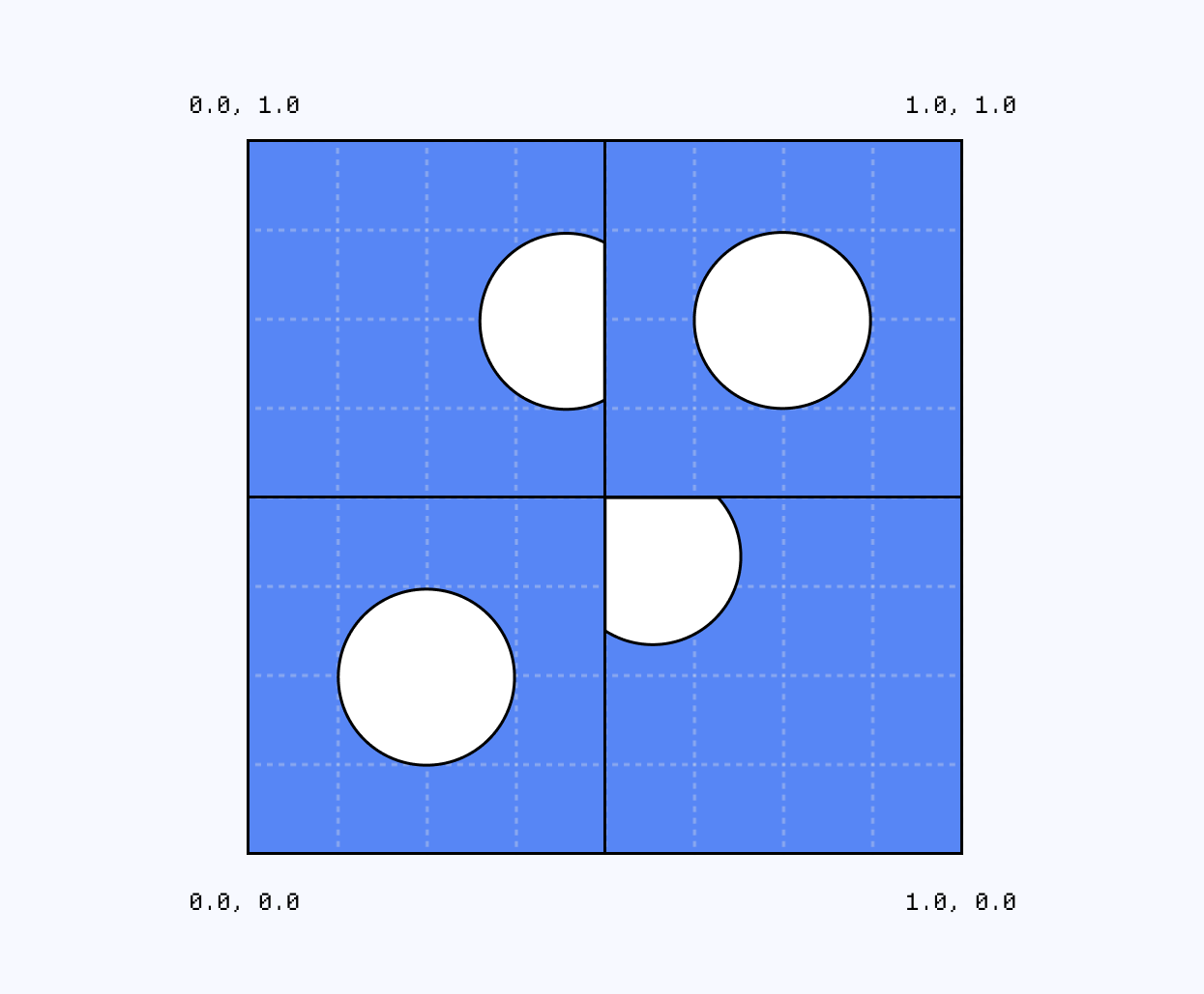
Instead of each pixel being aware of its own cell, we need to tweak our implementation and start looking at the neighboring cells as well. By checking a 3x3 area around the current pixel, we can allow the dots to leak across cells without being clipped.

1
vec2 pixelCoord = vUv * uResolution;
4
vec2 baseCellIndex = floor(pixelCoord / uPixelSize);
6
vec4 finalColor = vec4(0.0);
10
const int searchRadius = 1;
12
for (int dx = -searchRadius; dx <= searchRadius; dx++) {
13
  for (int dy = -searchRadius; dy <= searchRadius; dy++) {
14
    vec2 cellIndex = baseCellIndex + vec2(float(dx), float(dy));
15
    vec2 cellCenter = (cellIndex + 0.5) * uPixelSize;
17
    vec2 uvPixel = cellCenter / uResolution;
18
    vec4 texColor = texture(uTexture, uvPixel);
20
    float dist = length(pixelCoord - cellCenter);
22
    float radius = uPixelSize * uRadius;
24
    float aa = fwidth(dist);
25
    float circle = 1.0 - smoothstep(radius - aa, radius + aa, dist);
27
    if (circle > maxCircle) {
29
      finalColor = texColor;
34
vec3 bgColor = vec3(0.0);
35
vec3 color = mix(bgColor, finalColor.rgb, maxCircle);

• We introduce a nested loop that searches at a 1-cell radius around the current position.

• We define a baseCell as our current cell for the current pixel our fragment shader is processing.

• We calculate the cellCenter of each neighbor in the 3x3 kernel. This allows us to measure the distance dist between the current pixel and all the neighboring cell centers.

• We check the reachability. We sample the color at that neighbor’s center to determine the dot's color and check if that specific neighbor's dot is large enough to "reach" our current pixel.

• Many neighboring circles may reach our current pixel; we need to ensure we only have one winner, and this is why we store the “biggest” circle in maxCircle.

This is the mechanism that erases the clipping, as now every cell can get part or all of its pixels colored based on the influence of its neighboring cells. We can do many things with this, the first one being increasing the size of our circles beyond the cell’s size, which yields a beautiful, almost watercolor-y output.

Gooey halftone

What if we could make our dots look like ink? Or make them look more liquid by simulating some sort of surface tension between neighboring dots?

Now that we know how to render halftone dots beyond their grid cells, there’s nothing preventing us from doing so! By adding leveraging luma-based radius for our dots, as well as blending overlapping circles with a smoothmin function ⁵, we can make our dots look more liquid, as if they had some kind of surface tension:

These two small changes allow neighboring circles that are close enough to one another to gracefully merge as if they were ink drops. This yields a more organic-looking halftone variant, one that shines when overlayed on top of an animated 3D scene, as showcased in the demo below, which also features the full code.

Displaced dots

As a final variant of halftone, I wanted to take the time to look into ways we could make the effect more dynamic / alive by allowing the dots to be animated and move. We pretty much have the recipe already in place to achieve this through the two previous examples, and all we need now is a good idea to implement.

On my end, my original source of inspiration for this section was this artwork by @adamfuhrer, a visual artist I’m a big fan of.

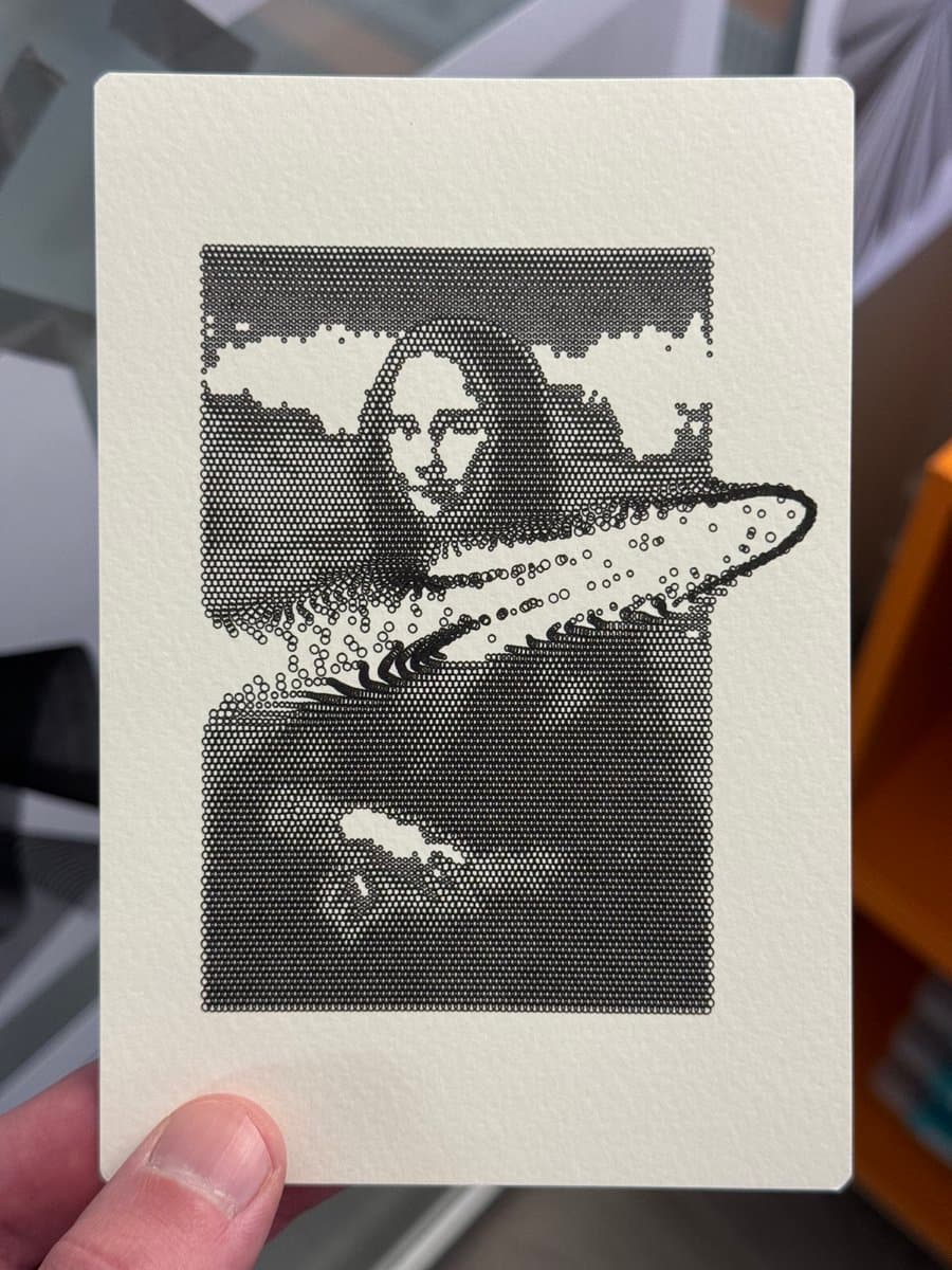
1. It’s leveraging the ring halftone pattern we saw in the first part of this article.

2. We have some rings positioned way beyond their original position, which means we’ll need a relatively large kernel when rendering our effect.

3. There’s the trail left by a swooping movement across the rings. This is what we have yet to implement!

For this experiment, I reused the MouseTrail component I originally built for the Pixelated Mouse Trail effect demo of my post-processing article. As it did for that effect, this standalone component renders the trail of the user’s cursor through:

• Two Frame Buffer Objects (FBOs) and ping pong rendering

• The position and velocity of the cursor.

It is rendered off-screen, and its resulting texture is passed directly to our halftone effect as a uniform. Once sampled, we can get the brightness of the red and green channels, representing the cursor movement alongside the x and y axes, to know the direction and intensity of the displacement.

1
vec2 brushUV = cellCenter / resolution;
2
vec4 brush = texture2D(brushTexture, brushUV);
3
vec2 brushVel = clamp(brush.rg, -0.45, 0.45);
4
float brushIntensity = length(brushVel);
6
vec2 forwardDir = brushIntensity > 0.001 ? brushVel / brushIntensity : vec2(0.0);
7
vec2 perpDir = vec2(-forwardDir.y, forwardDir.x);
8
float side = sign(random(cellCenter) - 0.5);
10
float t = smoothstep(0.0, 0.5, brushIntensity);
11
float easeIn = t * t * t;
12
float easedIntensity = mix(easeIn, t, 0.5);
14
vec2 srcUV = clamp(cellCenter / resolution, 0.0, 1.0);
15
vec3 srcColor = texture2D(inputBuffer, srcUV).rgb;
18
vec2 displacement = forwardDir * 0.75 + perpDir * side * 0.25;
20
cellCenter += displacement * mouseStrength * easedIntensity;

The displacement is then applied to the center of the neighboring cells to shift where the dots/rings are visually rendered. This creates the illusion of movement, which in this case is defined as follows:

• We first define the direction of the movement: vec2 forwardDir = brushIntensity > 0.001 ? brushVel / brushIntensity : vec2(0.0);

• We get the perpendicular vector to the direction: vec2 perpDir = vec2(-forwardDir.y, forwardDir.x);

• Pick a random side the ring will move towards perpendicularily

• Combine and ease the movement. In our case, it’s more weighted towards moving forward (75%) than on the sides (25%), giving the impression of the rings being gently pushed and slowly drifting sideways

Once again, this implementation is built on top of what we saw in the first subsection and consists of only a few tactical tweaks. I highly encourage exploring further what can be done with such a pattern.

As you can see, from a very simple shape like a circle, we can quickly branch off to a diverse set of effects, each more interesting and pleasing than the other. This is also represented in code, as I managed to keep my shaders modular throughout my experiments, reusing the same functions from very simple effects to the more complex ones.

I had a lot of fun writing about my little halftone side quest, as the topic was on my list for quite some time now. I hope this article will serve you well to either introduce you to an accessible application of shaders or to wrap your head around some of the more tedious concepts. It will most likely serve as a base for another article this year that I plan to write on the topic of real-time shader-based paintings were from simple dots randomely rendered on the screen we can get to a shader capable of emulating different types of painting styles like impressionism, pointillism, and watercolor. The building blocks for this shader are very similar to those introduced here, which once again goes to show the versatility of halftone. This will be for another time, though! In the meantime, I’ll leave you with a teaser of what to expect.