One of the first things we teach our children growing up is how to group toys by colors, shapes, and sizes. Grouping objects into categories is a fundamental tool we use to understand the world around us. It's so important that we've developed several computational methods to find groups or patterns in data, and they are studied under a sub-field of machine learning called cluster analysis. There are several clustering algorithms, but k-means — the algorithm we're going to implement from scratch in Python and Mojo🔥 in this blog post — is one of the most popular due to its simplicity and ease of implementation.

In this blog post, I’ll:

• Explain what k-means is, how it works, and how to use it.
• Show you how to write the k-means clustering algorithm from scratch in Python and Mojo and highlight key differences between the two implementations.
• Guide you through code changes you'll need to make to port Python code to Mojo🔥 for significant performance benefits.

My goal is to introduce Mojo🔥 to Python developers using an example-driven workflow. This post will not make you a Mojo🔥 expert, but it will help you appreciate the similarities between Python and Mojo🔥 code, and how you can translate Python code to Mojo🔥 by introducing Mojo🔥 specific features like strong typing and vectorization to achieve substantial speedups over Python+NumPy code.

Get the code: All the resources shared in this blog post, including the complete implementation of k-means in Python and Mojo with detailed comments, scripts to run the examples, a benchmarking script, and utility functions that generate scatter plots (like the one below) and benchmark plots, are all available on GitHub:

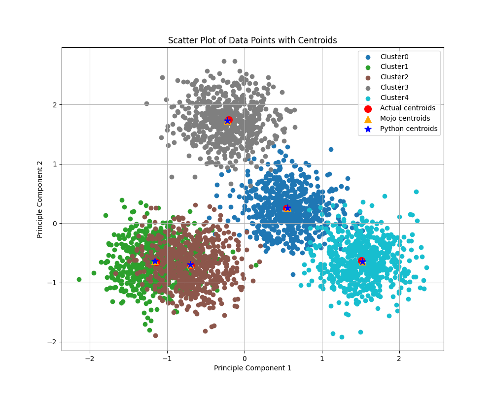
The figure below shows clusters calculated by our Python+NumPy and Mojo implementations, within a synthetically generated dataset containing 3,000 samples (rows) and 100 features (columns), grouped into five categories. In the past, I’ve struggled to visualize 100 dimensional data (believe me, I’ve tried), so I reduced the data to two dimensions using Principal Component Analysis (PCA). The actual centroids, along with those calculated using each implementation (shared in this blog post), are also shown.

k-means performance and benchmarking

In this blog post, I’ll share some benchmark comparisons to show performance improvements of k-means in Mojo🔥 over Python+NumPy implementation. Performance can depend on many factors. In the plot below (click to zoom), I illustrate the speedup achieved by Mojo🔥 k-means over Python+NumPy k-means by varying the (1) number of clusters, (2) number of samples, and (3) number of features, while keeping other variables constant as specified in the plot. We observe speedups ranging from 6x to 250x with Mojo🔥 (click to zoom, best viewed when browser is full screen):

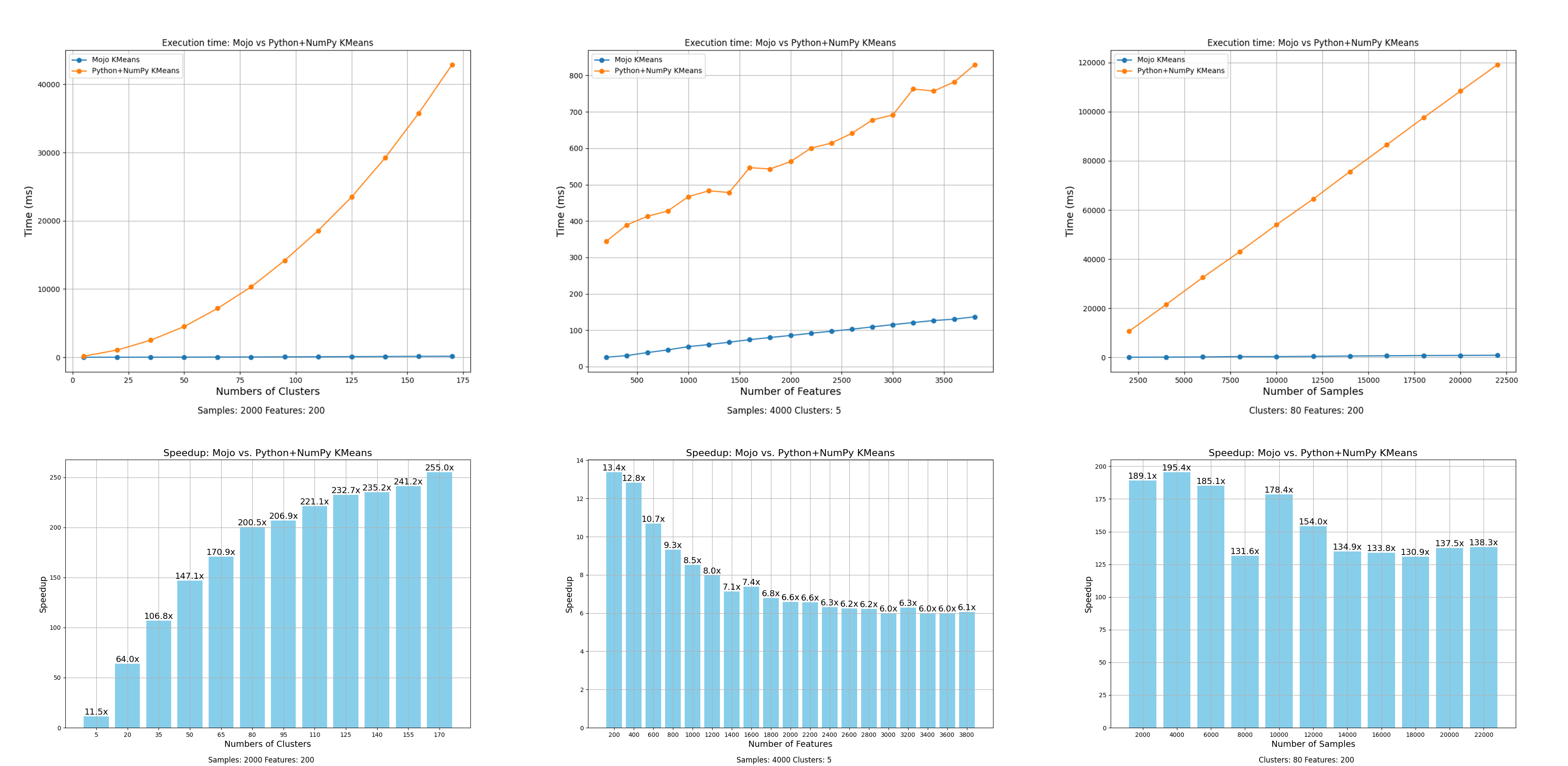
We'll discuss benchmarking in a little more detail at the end of this blog post, for now here are the key takeaways:

• Every workload is unique, so it’s hard to make generalized speedup statements, especially when comparing complex projects with small, specialized functions designed for benchmarking.
• For complex ML algorithms like k-means, several factors—such as dataset size, number of clusters, number of iterations, and the effectiveness of the code—contribute to performance.
• Porting Python+NumPy code to Mojo🔥 will offer considerable speedups, since computationally expensive parts can easily be vectorized and parallelized.

But you really came here for the code, and I won’t keep you waiting. Let’s jump right into the implementation. First, a basic summary of the k-means algorithm and its details—it’s not complicated, I promise.

What is k-means clustering? 

Consider a tabular dataset with M rows and N columns, where each row represents an N-dimensional data point, and there are M data points in total. K-means is an iterative algorithm that assigns each data point to its nearest cluster based on its distance to the centroid of that cluster. The algorithm recalculates the centroids iteratively to reduce the average within-cluster distance. Upon convergence, similar data points are grouped together in common clusters.

For example, in an e-commerce dataset, each column might represent customer attributes such as past purchase history and demographic data, while each row represents a different customer. K-means clustering can help you cluster customers together and determine if there are common buying preferences within a cluster. You can use this information to recommend similar products and services to customers in the same cluster.

The algorithm is very simple. For a given dataset and desired number of clusters k.

1. Initialization: Pick initial k centroids using k-means++ initialization algorithm (discussed below). 
2. Lloyd's iteration: Perform these steps till convergence:
   1. Assignment: For each data point calculate distance to each of the k centroids and assign the data point to the closest centroid.
   2. Update: For each cluster, recalculate the centroid by computing the mean of all data points assigned to that cluster.

In flow chart form:

K-means class definition in Python and struct definitions in Mojo

I’ll discuss k-means++ algorithm, Lloyd’s iteration and convergence criterion in more detail along with the Python and Mojo code below. Let’s now a look at the skeleton of both Mojo 🔥 implementation and Python implementation side by side (click to zoom, best viewed when browser is full screen):

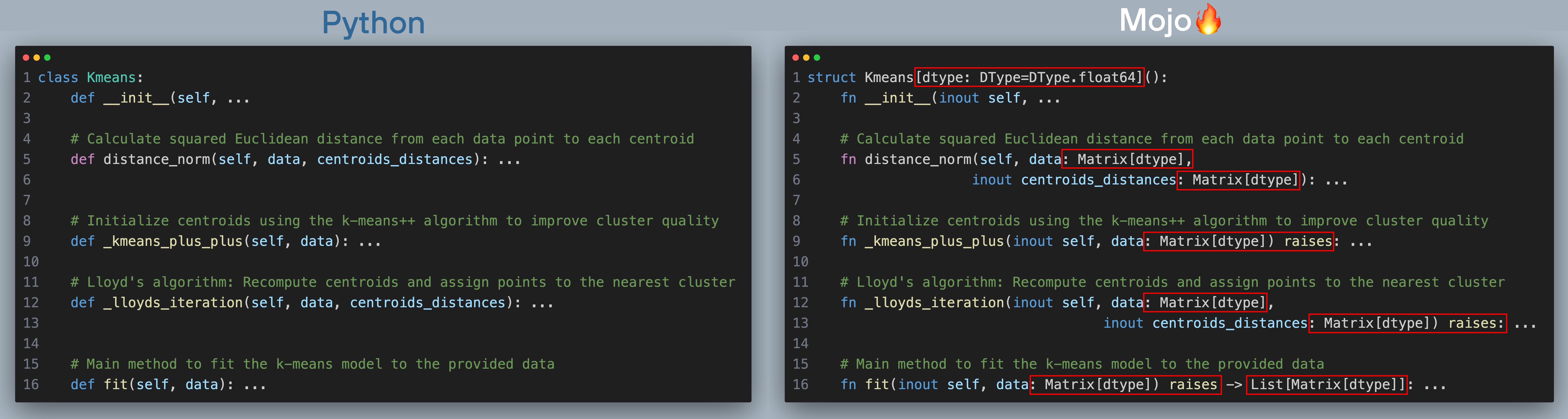
At a high level you should observe:

• In Python we define a class and in Mojo🔥 we define a struct
• All the functions names are the same: __init__, distance_norm, _kmeans_plus_plus, fit
• Function arguments in Mojo are typed and they are not in Python.
• fit function have return type specified
• Some function arguments have a keyword inout in front of their name

If you are a seasoned Mojician🪄all this makes perfect sense to you. If you are a Python Wizard 🧙, Mojo code might look very similar to typed Python code. Unlike Python however, Mojo is a compiled language and even though you can still use def for functions and omit types like in Python, Mojo lets you declare types so the compiler can better optimize code, and improve performance. We want to make k-means ⚡fast⚡ so I chose to use Mojo🔥 native features to speed it up. Both can be used the exact same way. 

In Mojo:

In Python:

In scikit-learn:

I’ve written both the Python and Mojo versions to be very similar to k-means implementation in scikit-learn:

The terminal output when running all three using the run_kmeans.mojo file in GitHub is below.

For this specific problem configuration where n_clusters = 5, n_samples =  3000, and n_features =  100, Mojo is faster than both our Python implementation and scikit-learn’s implementation by 13 and 6 times respectively, with all of them converging close to a similar final inertia value. Scikit-learn’s implementation converges in only 3 iterations, and yet Mojo k-means is faster even when running for 3 extra iterations. If you’re wondering why scikit-learn converges in fewer iterations, it could be one of these reasons:

1. Certain random initial centroids may be closer to the final centroid, and therefore help converge sooner.
2. Scikit-learn’s k-means implements multiple convergence criteria, whereas our implementation only checks for change in inertia value.

Now let’s compare each section of the code side by side starting with class definition in Python and struct definition in Mojo and their initialization dunder method __init__(). We define all of k-means hyperparameters and algorithm options here (click to zoom, best viewed when browser is full screen). The red boxes show what changes we needed to make to port code over to Mojo.

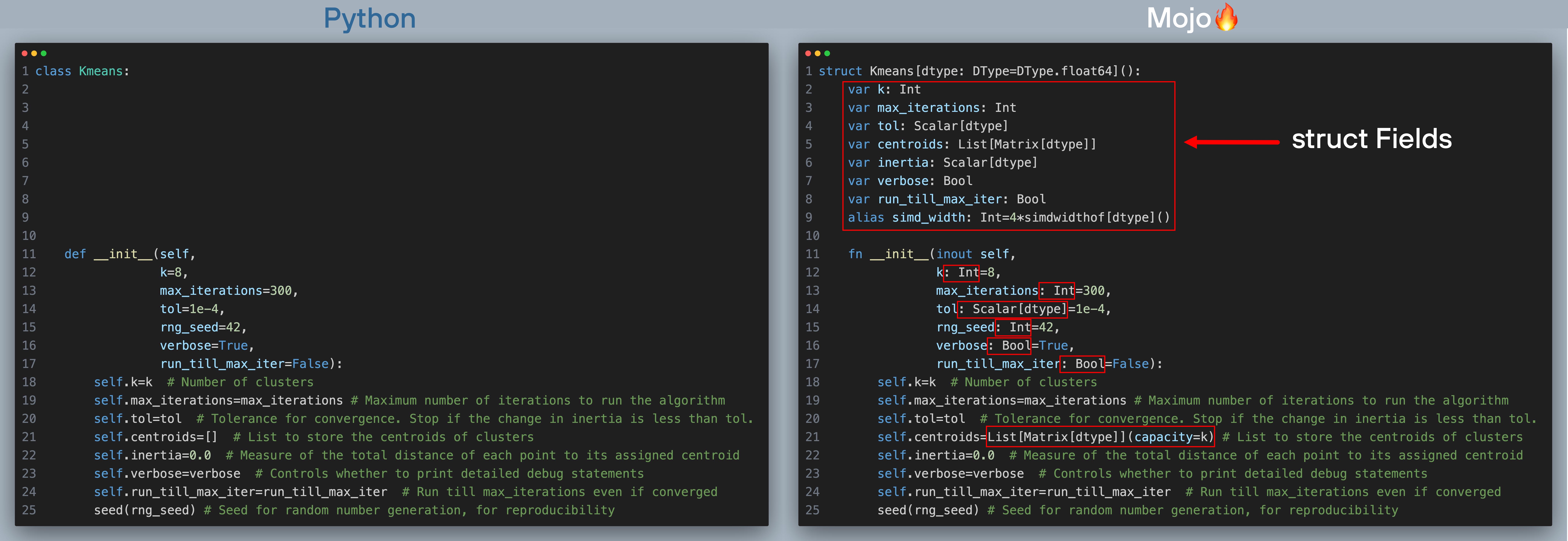
To port the Python class definition over to Mojo struct, you’ll need to make a few minor changes. 

• __init__() is mostly unchanged. The only modifications you’ll need to make is to add types to all arguments to __init__(). The variable self.centroids is an empty list in Python which can grow dynamically, whereas in Mojo structs are static and compile-time bound, so we declare self.centroids to be a list with a fixed capacity, equal to number of clusters.
• The struct definition itself differs from the Python class definition. We declare struct just like a Python class, but since structs are static and compile-time bound, parameterized by dtype which defaults to Float64. We also define struct Fields which are initialized in the __init__() function.

For more detailed comparisons between Mojo structs and Python classes see this documentation page.

k-means fit() function in Python+NumPy and Mojo

Now, let’s move on to the fit() function which runs the k-means clustering algorithm (click to zoom, best viewed when browser is full screen). The red boxes show what changes we needed to make to port code over to Mojo.

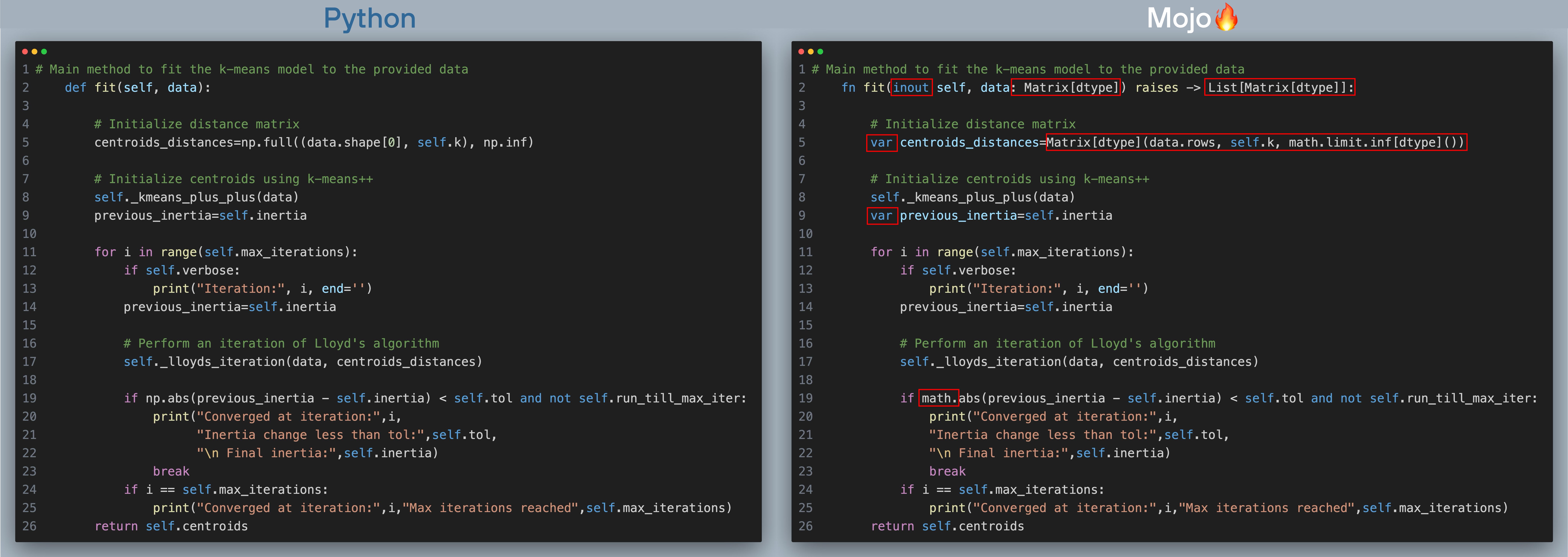
The fit function implements this updated flow chart below. I’ve added line numbers (which are the same for Python and Mojo implementations), next to the corresponding step in the flowchart.

In the next section we’ll learn more about each of these steps, for now let’s summarize the changes in fit() going from Python -> Mojo:

• We use fn instead of def for our struct methods. While Mojo supports the same dynamism and flexibility as a Python def function, fn functions provide strict type checking and additional memory safety, which can lead to faster performance.
• We add types to all function arguments and specify the return type.
• fn functions require variables to be declared with var 
• We replace NumPy’s np.abs and np.inf with Mojo standard library’s math.abs and math.limit.inf

Simple enough? Sure is! but let's address the elephant 🐘in the room: NumPy.

Python has NumPy, a powerful library for numerical computing that implements high-performance matrix operations. This library has been in development for more than 20 years and implements most of its high-performance routines directly in C to maximize hardware utilization. Mojo, on the other hand, is a younger language and lacks an equivalent high-performance matrix library.

I've implemented a Matrix data structure in Mojo, which provides rudimentary, NumPy-like basic matrix operations such as slicing, reductions, and element-wise mathematical operations in a fast, vectorized manner. You’ll see that all the NumPy references in the Python k-means code are replaced by Matrix in the Mojo k-means code. For example, in the function definition for fit(), you'll see that data has a type Matrix[dtype].

Note on convergence criteria (Lines 19 and 25 in the code excerpt): Since k-means is an iterative algorithm, we have to implement conditions to break from the iteration loop. In our example, we'll check for two convergence criteria: (1) the maximum number of iterations is reached, and (2) the change in inertia is below a certain threshold. In the k-means algorithm, inertia refers to the total sum of squared distances between each data point and the centroid of the cluster to which it is assigned.

k-means plus plus initialization in Python+NumPy and Mojo

Since k-means is an iterative algorithm, we must start with some initial centroids and iteratively improve them. This also means the algorithm is sensitive to the initial selection of centroids, and poor initialization can lead it to converge to local minima, resulting in suboptimal clusters. Rather than starting with random centroids, the k-means++ algorithm provides better initial centroids that are more evenly distributed, resulting in faster convergence. Below are the Python and Mojo implementations of the k-means++ algorithm (click to zoom, best viewed when browser is full screen). The red boxes highlight the changes we needed to make to port the code over to Mojo.

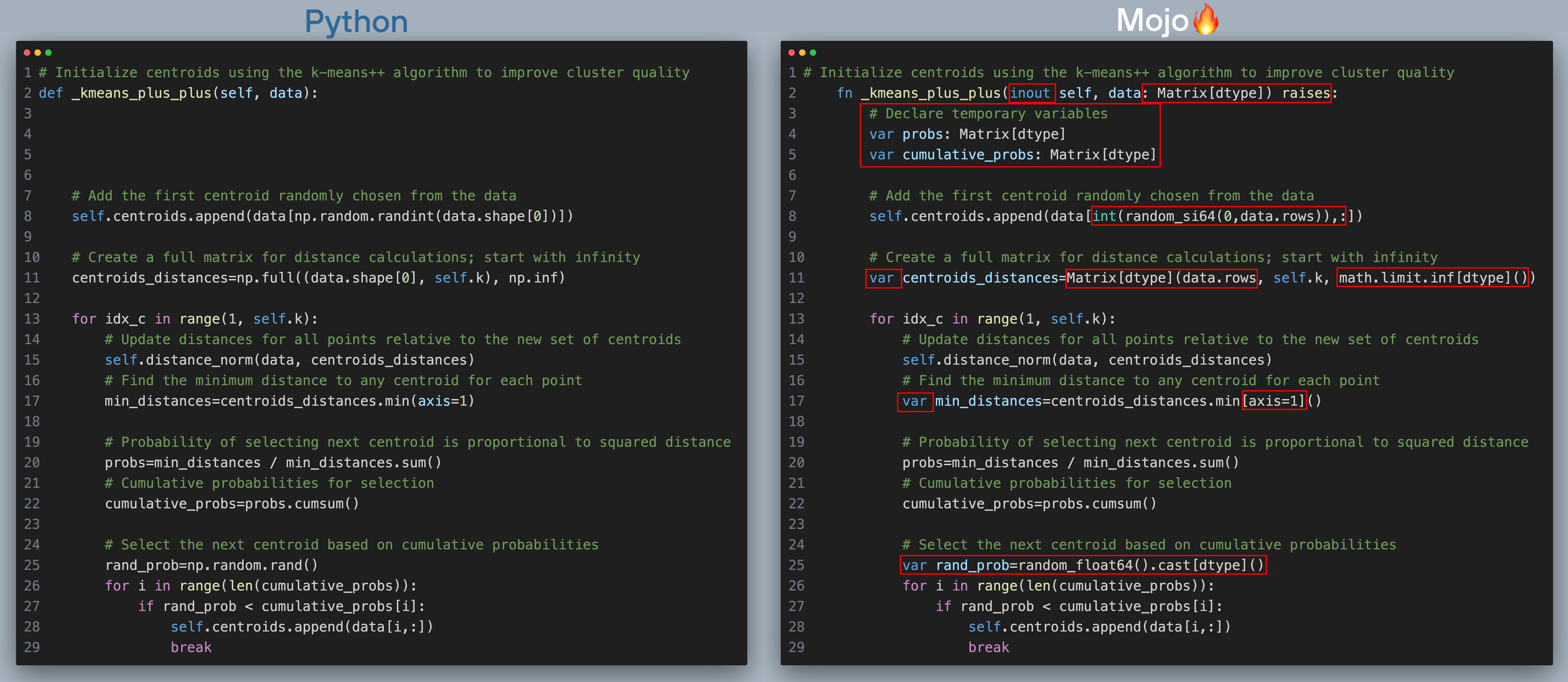
Here’s what's happening in the above code with corresponding line number in the code excerpt:

• [Line 8] Choose one data point uniformly at random from data as the first centroid
• [Line 13] Iteratively find remaining k-1 centroidssome text
  • [Line 15] For each data point in data, compute squared Euclidean distance between the point and all found centroids
  • [Line 17] Find the minimum distance to any centroid for each data point
  • [Line 20 - 29] Choose one new data point at random as a new centroid, using a weighted probability distribution where a new centroid is chosen with probability proportional to squared Euclidean distance to centroid.
  • Repeat till k initial centroids are found 

Now let’s summarize the changes in _kmeans_plus_plus() going from Python -> Mojo:

• We again use fn functions instead of def.
• We declare all variables with var
• We declare temporary variables in Mojo for faster performance.
• We use random_si64 from the Mojo math standard library to replace NumPy’s np.random.randint
• We replace np.full in the Python code with Matrix[]() in Mojo the code
• We replace np.random.rand() in the Python code with random_float64() from the Mojo math standard library in the Mojo code

Lloyd’s iteration in Python+NumPy and Mojo

In the k-means algorithm, Lloyd's iteration performs two steps:

1. Cluster assignment: For each data point in the dataset, calculate its distance to each centroid. Assign each data point to the cluster whose centroid is closest to it.
2. Centroid updates: After assigning all data points to clusters, recalculate the centroids as the mean of all data points assigned to each cluster.

Below is Python and Mojo implementation of k-means plus plus algorithm (click to zoom, best viewed when browser is full screen). The red boxes show what changes we needed to make to port code over to Mojo.

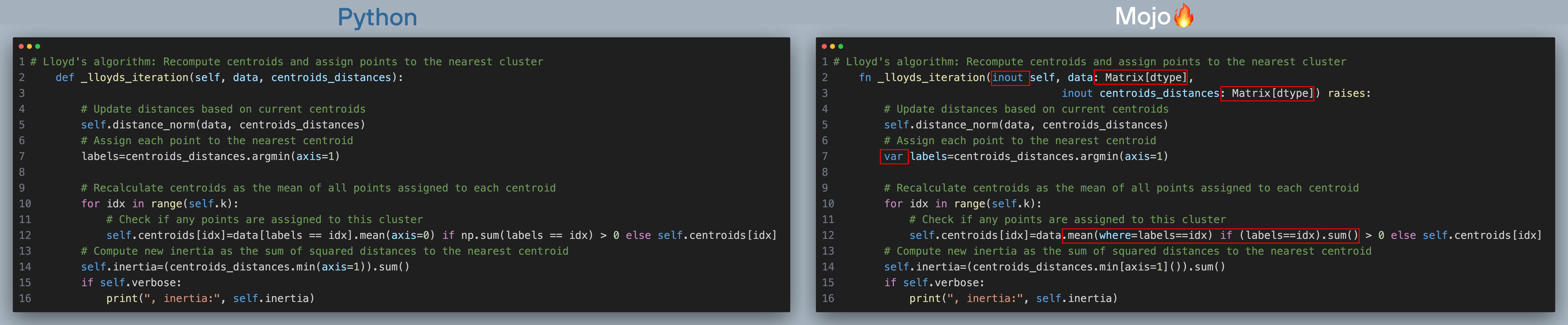
Here’s what's happening in the above code with corresponding line number in the code excerpt:

• [Line 5] For each data point in the dataset, calculate its distance to each centroid.
• [Line 7] Assign each data point to the cluster whose centroid is closest to it.
• [Line 10 - Line 12] Recalculate the centroids as the mean of all data points assigned to each cluster.
• [Line 14] Calculate inertia

Now let’s summarize the changes in _lloyds_iteration() going from Python -> Mojo:

• We added types to function arguments
• We declare all variables with var
• We replaced NumPy operations to calculate mean and sum with Matrix[]() equivalent in Line 12

We’re at the home stretch here! Let’s take a look at our final function.

Calculating squared Euclidean distance Python+NumPy and Mojo

The most computationally intensive part of the k-means algorithm is typically the cluster assignment step which involves calculating the distance between each data point and each centroid to determine which centroid is closest to each point. Accelerating the distance calculation can significantly speed up each Lloyd’s iteration step and k-mean clustering as a whole.

While Python relies on NumPy’s fast implementation of Euclidean distance calculation implemented in C language and exposed via np.linalg.norm(). In Mojo we’ll implement this from scratch by tapping into the full power of Mojo’s ease of use vectorization and parallelization support. In this section Python and Mojo code will look nothing alike (but if you are free to imagine a big blob of C code that you trust, has got your back).

Below is Python and Mojo implementation of k-means plus plus algorithm (click to zoom, best viewed when browser is full screen). The red boxes show what changes we needed to make to port code over to Mojo.

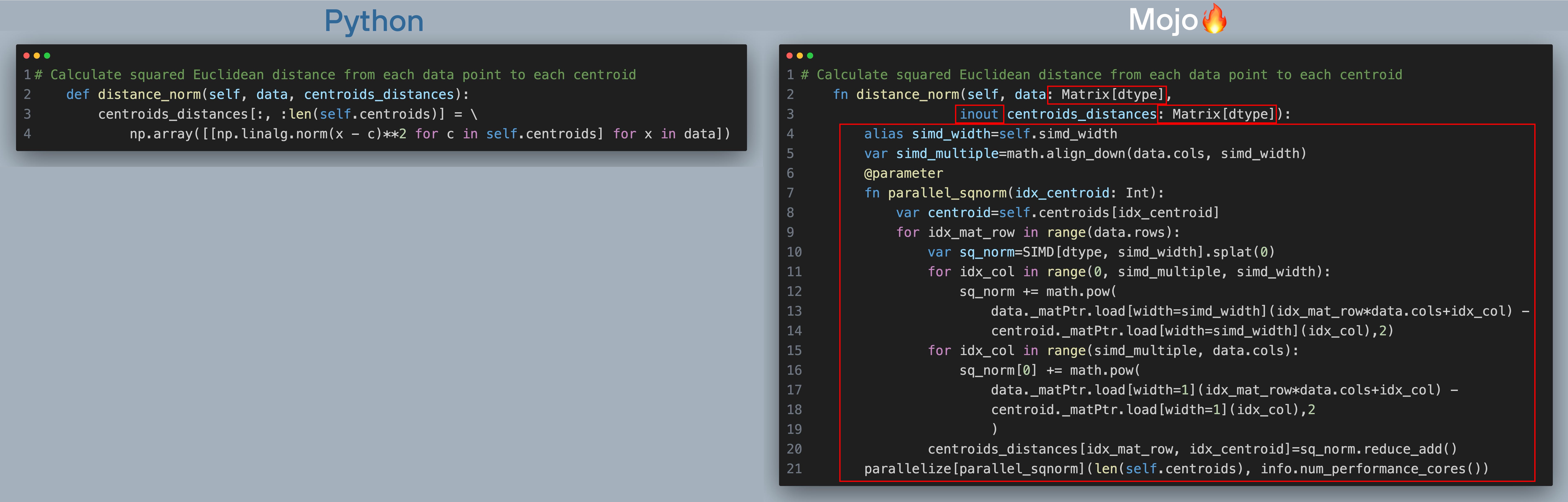
Here’s what's happening in the above code with corresponding line number in the code excerpt:

• [Line 2] In the function definition we added the inout keyword infront of centroids_distance to receive a reference to the data structure that is mutable. i.e. changes to centroids_distance will be reflected outside the function, so we don’t need to make copies of the data structure. NumPy arrays work this way by default in Python.
• [Line 7] defines a closure that calculates distance between all data points in data to the centroid/cluster number idx_centroid in the argument. Writing a function this way enables us to call Mojo’s parallelize function, so we can calculate centroid distances for each cluster in parallel.
• [Line 8] starts the outer loop that iterates over rows of data and calculates the distance between the data points in loop variable idx_mat_row and the current centroid in idx_centroid.
• [Line 11 - Line 19] includes the inner loops that calculate the squared norm between the data points in idx_mat_row of data and data points in centroid number idx_centroid, in a vectorized way. By operating on simd_width elements simultaneously, we can get huge speedup depending on the value of simd_width on your system. Since simd_width is a power of 2 we include a second loop on line 15 to processes the elements from floor(data.cols / simd_width) * simd_width to data.cols

 Now let’s summarize the changes in distance_norm() going from Python -> Mojo:

• We implemented vectorized and parallelized squared Euclidean norm calculation from scratch.
• We leveraged SIMD (Single Instruction, Multiple Data) operations using special CPU registers that can process multiple bits of data at the same time.

Phew.

If you are a Python developer with no background in system’s programming languages like C or C++ the code above was probably hard to follow. I could have alternatively written a much simpler looking loop that didn’t take advantage of vectorization and parallelization to make it look like Python code, by trading off some performance. But therein lies the beauty of Mojo. You can write code that looks like Python for non-performance critical code and roll up your sleeves and write low-level code when performance matters. Mojo🔥 meets you where you are.

Running and benchmarking both Python+NumPy and Mojo k-means implementations

The example on GitHub includes two files to test our implementations: run_kmeans.mojo and bench_kmeans.mojo.

run_kmeans.mojo 

This file shows you how to create some test data with a specified number of clusters and cluster it using Python+NumPy, Mojo and scikit-learn implementation of k-means. It also includes an option to generate 2-dimensional scatter plots of the 1st and 2nd principal components to visualize high-dimensional data. Here is a simple example of how to cluster some synthetic data with n_samples = 3000, n_features = 200 and n_clusters = 10 generated using scikit-learn's make_blobs function. 

Partial output:

You can see that all three implementations converge to a similar final inertia value. You will, however, see run-to-run variations due to the inherent randomness of the k-means algorithm.

bench_kmeans.mojo

This file implements a very simple benchmarking setup to compare the performance of Python+NumPy, Mojo, and scikit-learn implementations of k-means. It also generates benchmarking plots shown below (click to zoom). To test the performance of both implementations, in bench_kmeans.mojo we specify the ranges of values to sweep for the benchmark. When we sweep one variable, we keep the other two constant and plot the results.

Note that the ranges and the choice of variable values that are held constant are arbitrary. Feel free to run bench_kmeans.mojo with different ranges and measure performance. Since the k-means algorithm is sensitive to random initial centroids, one implementation may converge sooner than the other, potentially running much quicker. To make the comparison fairer, we can set the k-means argument run_till_max_iter=True, which will force the algorithm to run until max_iterations even if the convergence criterion has been met.

Below, you can see plots of the time taken to run until the default max_iterations = 10 when sweeping cluster size, number of samples, and number of features. The values that are held constant are displayed at the bottom of each plot. For these ranges, we observe speedups ranging from 6x to 250x when using Mojo🔥. Each experiment runs for 10 full iterations with other convergence criteria disabled, providing a fair comparison of performance. In our implementation, I noticed that:

1. In Plot 1, scaling the number of clusters results in higher speedups, since we compute the distance between data points and clusters much more frequently. Mojo🔥's vectorized and parallelized code is significantly faster at computing distances.
2. In Plot 2, scaling the number of samples shows a more consistent distribution, with a median speedup of approximately 150x.
3. In Plot 3, scaling the number of features results in a decreasing speedup as the number of feature columns increases, due to the limited number of cores available on my MacBook Pro with M2 Pro. I expect that on a system with more cores, the speedup would be consistent.

Click to zoom, Best viewed when browser is full screen:

Conclusion

I hope you enjoyed reading this primer on the k-means algorithm and how you can translate computationally intensive code from Python to Mojo🔥 for faster performance. Building an end-to-end example like this k-means clustering implementation is a great way to learn how to use a new programming language. 

Please take this code, modify it, test it and run your own experiments with it. You can also use it to implement other ideas using the building blocks from this example. One cool example could be k-nearest neighbor search for Retrieval Augmented Generation (RAG) applications which also relies on fast euclidean Distance calculations. Join our Discord community and share your projects with other Mojicians🪄!

Thank you for reading! Here are some additional resources to get started. 

• Get started with downloading Mojo
• Head over to the docs to read the programming manual and learn about APIs
• Explore the examples on GitHub
• Join our Discord community
• Contribute to  discussions on the Mojo GitHub
• Read and subscribe to Modverse Newsletter 
• Read Mojo blog posts, watch developer videos and past live streams
• Report feedback, including issues on our GitHub tracker

Until next time🔥!