PyTorch-26H-4
主页:https://www.freecodecamp.org/news/learn-pytorch-for-deep-learning-in-day/
youtub:https://youtu.be/V_xro1bcAuA
github:https://github.com/mrdbourke/pytorch-deep-learning
Learn PyTorch for Deep Learning: Zero to Mastery book:https://www.learnpytorch.io/
PyTorch documentation:https://pytorch.org/docs/stable/index.html
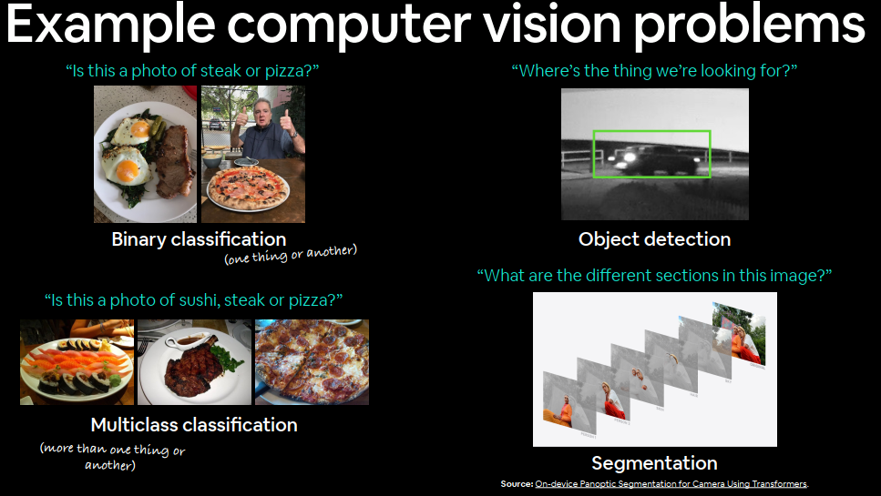
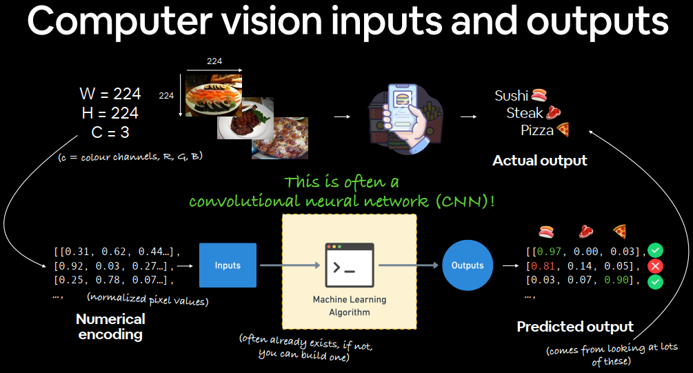
计算机视觉Computer vision 是教计算机看东西的艺术。
例如,它可能涉及建立一个模型来对照片是猫还是狗进行分类(二元分类binary classification )。
或者照片是猫、狗还是鸡(多类分类multi-class classification )。
或者识别汽车在视频帧中出现的位置(物体检测object detection )。
或者弄清楚图像中不同物体可以分离的位置(全景分割panoptic segmentation )。
machinelearning_apple
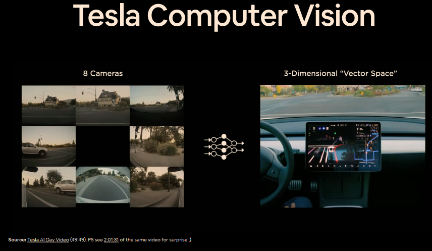
如果您使用智能手机,那么您已 经使用了计算机视觉。
相机和照片应用程序使用计算机视觉来增强computer vision to enhance 和分类图像。
现代汽车使用计算机视觉computer vision 来避开其他车辆并保持在车道线内。
制造商使用计算机视觉来识别各种产品的缺陷。
安全摄像机使用计算机视觉来检测潜在的入侵者。
本质上,任何能够用视觉描述的事物都可能成为潜在的计算机视觉问题。
torch.nn.Conv2d
Getting a vision dataset to work with using torchvision.datasets
使用 torchvision.datasets 获取视觉数据集
Architecture of a convolutional neural network (CNN) with PyTorch
使用 PyTorch 构建卷积神经网络 (CNN) 架构
An end-to-end multi-class image classification problem
端到端多类图像分类问题
Steps in modelling with CNNs in PyTorch
使用 PyTorch 中的 CNN 建模的步骤
Creating a CNN model with PyTorch
使用 PyTorch 创建 CNN 模型
Picking a loss and optimizer
选择损失和优化器
Training a PyTorch computer vision model
训练 PyTorch 计算机视觉模型
Evaluating a model
评估模型
话题
内容
0. PyTorch 中的计算机视觉库
PyTorch 有许多内置的有用的计算机视觉库
1. 加载数据
为了练习计算机视觉,我们将从FashionMNIST](https://github.com/zalandoresearch/fashion-mnist)中的一些不同服装的图像开始。
2.准备数据
我们有一些图像,让我们用 PyTorch DataLoader 加载它们,以便我们可以在训练循环中使用它们。
3. 模型 0:建立基线模型
在这里我们将创建一个多类分类模型来学习数据中的模式,我们还将选择一个损失函数 loss function 、优化器 optimizer 并建立一个训练循环training loop .。
4. 做出预测并评估模型 0
让我们用基线模型做出一些预测并对其进行评估。
5. 为未来型号设置与设备无关的代码
编写与设备无关的代码是最佳做法,因此让我们进行设置。
6. 模型 1:添加非线性
实验是机器学习的重要组成部分,让我们尝试通过添加非线性层来改进我们的基线模型。
7.模型2:卷积神经网络(CNN)
是时候具体了解计算机视觉并介绍强大的卷积神经网络架构了。
8. 比较我们的模型
我们建立了三个不同的模型,让我们对它们进行比较。
9.评估我们的最佳模型
让我们对随机图像做出一些预测并评估我们最好的模型。
10. 制作混淆矩阵
混淆矩阵是评估分类模型的好方法,让我们看看如何创建一个混淆矩阵。
11.保存并加载性能最佳的模型
因为我们可能需要稍后使用我们的模型,所以我们保存它并确保它能正确加载。
PyTorch 计算机视觉库
torch.utils.data.Dataset和类torch.utils.data.DataLoader不仅适用于 PyTorch 中的计算机视觉,它们还能够处理许多不同类型的数据。
torchvison文档
导入相关依赖项:
1
2
3
4
5
6
7
8
9
10
11
12
13
14
15
import torchfrom torch import nnimport torchvisionfrom torchvision import datasetsfrom torchvision.transforms import ToTensorimport matplotlib.pyplot as pltprint (f"PyTorch version: {torch.__version__} \ntorchvision version: {torchvision.__version__} " )
1
2
PyTorch version: 2.4.1 torchvision version: 0.19.1
从 FashionMNIST 开始。
MNIST,Modified National Institute of Standards and Technology,修改后的国家标准与技术研究院
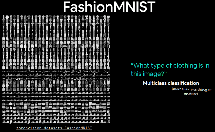
original MNIST dataset 原始 MNIST 数据集包含数千个手写数字示例(从 0 到 9),用于构建计算机视觉模型来识别邮政服务的数字。
FashionMNIST Zalando Research 制作的FashionMNIST是一个类似的设置。
包含 10 种不同服装的灰度图像。
torchvision.datasets包含大量示例数据集,可用于练习编写计算机视觉代码。FashionMNIST 就是其中一个数据集。由于它有 10 个不同的图像类别(不同类型的服装),因此它是一个多类别分类问题。
稍后,我们将构建一个计算机视觉神经网络来识别这些图像中不同风格的服装。
PyTorch 中存储了大量常见的计算机视觉数据集torchvision.datasets。
为了下载它,我们提供以下参数:
root: str,将数据下载到哪个文件夹?train: Bool,要训练还是测试分割?download: Bool,是否应该下载数据?transform: torchvision.transforms,想对数据进行哪些转换?target_transform, 如果您愿意,可以转换目标(标签)。
许多其他数据集torchvision都有这些参数选项。
1
2
3
4
5
6
7
8
9
10
11
12
13
14
15
16
train_data = datasets.FashionMNIST( root="data" , train=True , download=True , transform=ToTensor(), target_transform=None ) test_data = datasets.FashionMNIST( root="data" , train=False , download=True , transform=ToTensor() )
1
2
3
4
5
6
7
8
9
10
11
12
13
14
15
16
17
18
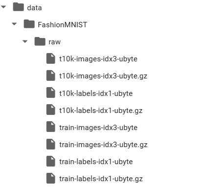
Downloading http://fashion-mnist.s3-website.eu-central-1.amazonaws.com/train-images-idx3-ubyte.gz Downloading http://fashion-mnist.s3-website.eu-central-1.amazonaws.com/train-images-idx3-ubyte.gz to data/FashionMNIST/raw/train-images-idx3-ubyte.gz 100% |██████████| 26.4M/26.4M [00:01<00:00, 14.2MB/s] Extracting data/FashionMNIST/raw/train-images-idx3-ubyte.gz to data/FashionMNIST/raw Downloading http://fashion-mnist.s3-website.eu-central-1.amazonaws.com/train-labels-idx1-ubyte.gz Downloading http://fashion-mnist.s3-website.eu-central-1.amazonaws.com/train-labels-idx1-ubyte.gz to data/FashionMNIST/raw/train-labels-idx1-ubyte.gz 100% |██████████| 29.5k/29.5k [00:00<00:00, 232kB/s] Extracting data/FashionMNIST/raw/train-labels-idx1-ubyte.gz to data/FashionMNIST/raw Downloading http://fashion-mnist.s3-website.eu-central-1.amazonaws.com/t10k-images-idx3-ubyte.gz Downloading http://fashion-mnist.s3-website.eu-central-1.amazonaws.com/t10k-images-idx3-ubyte.gz to data/FashionMNIST/raw/t10k-images-idx3-ubyte.gz 100% |██████████| 4.42M/4.42M [00:01<00:00, 4.32MB/s] Extracting data/FashionMNIST/raw/t10k-images-idx3-ubyte.gz to data/FashionMNIST/raw Downloading http://fashion-mnist.s3-website.eu-central-1.amazonaws.com/t10k-labels-idx1-ubyte.gz Downloading http://fashion-mnist.s3-website.eu-central-1.amazonaws.com/t10k-labels-idx1-ubyte.gz to data/FashionMNIST/raw/t10k-labels-idx1-ubyte.gz 100% |██████████| 5.15k/5.15k [00:00<00:00, 15.8MB/s]Extracting data/FashionMNIST/raw/t10k-labels-idx1-ubyte.gz to data/FashionMNIST/raw
国内下载有问题,使用google colab上传代码下载后加载到本地。
1 len (train_data),len (test_data)
查看第一个训练样本:
1
2
image, label = train_data[0 ] image, label
1
2
(tensor([[[0.0000, 0.0000, 0.0000, 0.0000, 0.0000, 0.0000, 0.0000, 0.0000,... , 9)
得到了一个很大的值张量(图像),它可以得出目标的单一值(标签)。
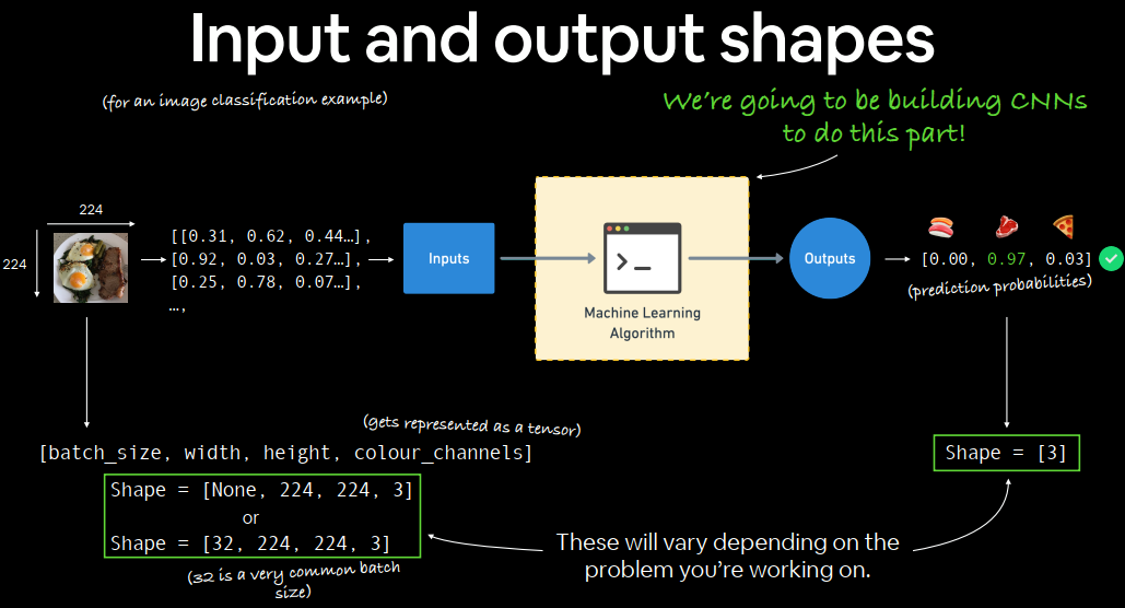
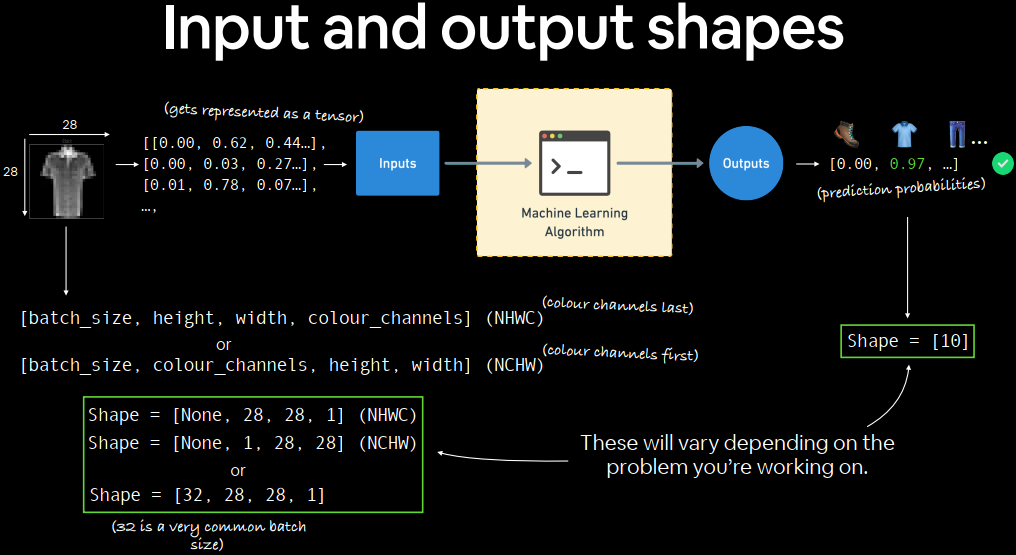
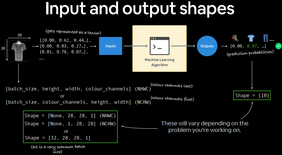
图像张量的形状[1, 28, 28]具体如下:
1 [color_channels=1, height=28, width=28]
有color_channels=1意味着图像是灰度的。
不同的问题会有不同的输入和输出形状。
如果color_channels=3,图像的像素值为红、绿和蓝(这也称为RGB 颜色模型)。
我们当前张量的顺序通常被称为CHW(颜色通道、高度、宽度)。
关于图像通道,channel last
关于图像应该表示为CHW(颜色通道优先)还是HWC(颜色通道最后)存在争议。NCHW和NHWC格式,其中N代表图像数量。例如,如果有batch_size=32,则张量形状可能是[32, 1, 28, 28]。我们稍后会介绍批量大小。NCHW(通道优先)作为许多运算符的默认设置。NHWC(通道最后)表现更好,被认为是最佳实践considered best practice .。
1
2
len (train_data.data), len (train_data.targets), len (test_data.data), len (test_data.targets)
1 (60000, 60000, 10000, 10000)
我们有 60,000 个训练样本和 10,000 个测试样本。
1
2
3
class_names = train_data.classes class_names
1
2
3
4
5
6
7
8
9
10
['T-shirt/top', 'Trouser', 'Pullover', 'Dress', 'Coat', 'Sandal', 'Shirt', 'Sneaker', 'Bag', 'Ankle boot']
10个类别的衣服,意味着多分类模型。
1
2
3
4
5
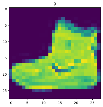
import matplotlib.pyplot as pltimage, label = train_data[0 ] print (f"Image shape: {image.shape} " )plt.imshow(image.squeeze()) plt.title(label);
1 Image shape: torch.Size([1, 28, 28])
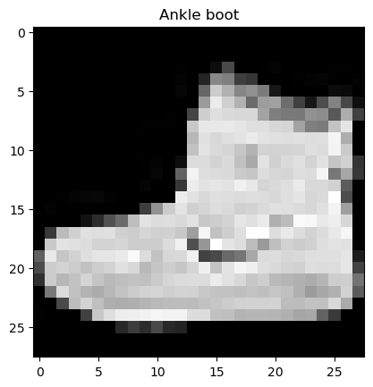
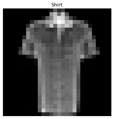
我们可以使用plt.imshow()的cmap参数将图像转换为灰度。
1
2
plt.imshow(image.squeeze(), cmap="gray" ) plt.title(class_names[label]);
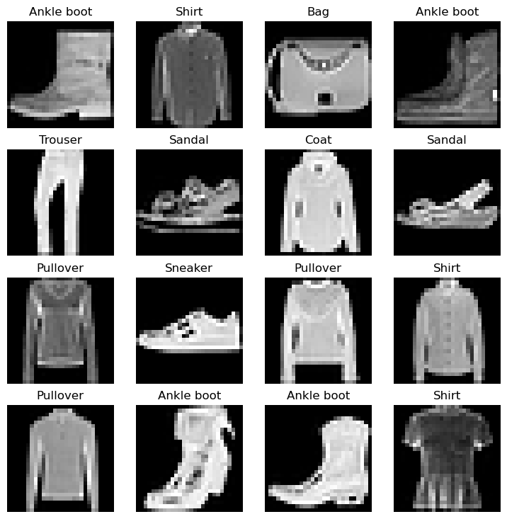
1 2 3 4 5 6 7 8 9 10 11 torch.manual_seed(42 ) fig = plt.figure(figsize=(9 , 9 )) rows, cols = 4 , 4 for i in range (1 , rows * cols + 1 ): random_idx = torch.randint(0 , len (train_data), size=[1 ]).item() img, label = train_data[random_idx] fig.add_subplot(rows, cols, i) plt.imshow(img.squeeze(), cmap="gray" ) plt.title(class_names[label]) plt.axis(False );
已经准备好数据集了,下一步是用torch.utils.data.DataLoader或准备。
它有助于将数据加载到模型中,用于训练和推理。
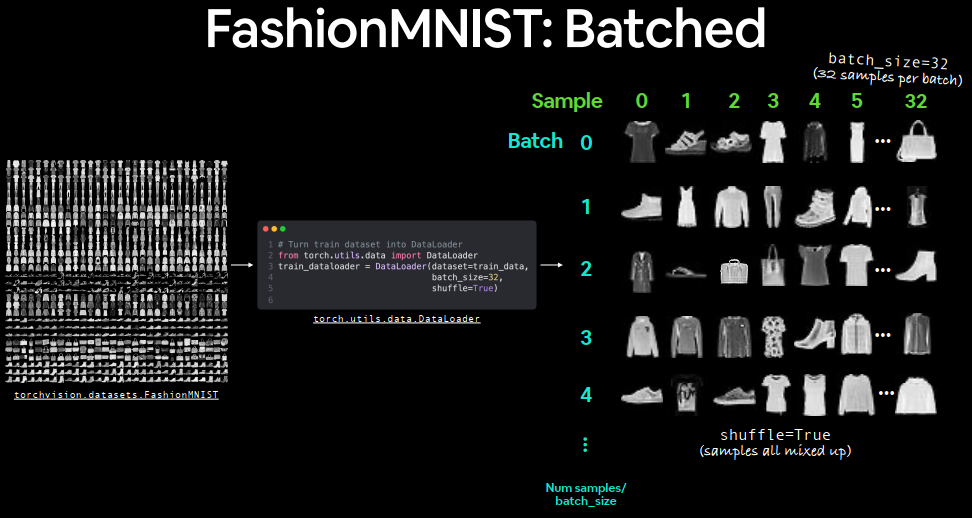
它将较大的数据转换 Dataset 成由较小块组成的 Python 可迭代数据。batch_size。
在理想世界中,您可以一次对所有数据进行前向传递和后向传递。
对于小批量(数据的一小部分),梯度下降在每个时期执行得更频繁(每个小批量一次,而不是每个时期一次)。合适的批次大小是多少?32 是一个好的起点
对 FashionMNIST 进行批处理,批处理大小为 32,并开启随机排序功能。其他数据集也会发生类似的批处理过程,但会根据批处理大小而有所不同。
torch.utils.data
1
2
3
4
5
6
7
8
9
10
11
12
13
14
15
16
17
18
19
20
from torch.utils.data import DataLoaderBATCH_SIZE = 32 train_dataloader = DataLoader(train_data, batch_size=BATCH_SIZE, shuffle=True ) test_dataloader = DataLoader(test_data, batch_size=BATCH_SIZE, shuffle=False ) print (f"Dataloaders: {train_dataloader, test_dataloader} " ) print (f"Length of train datalo ader: {len (train_dataloader)} batches of {BATCH_SIZE} " )print (f"Length of test dataloader: {len (test_dataloader)} batches of {BATCH_SIZE} " )
1
2
3
Dataloaders: (<torch.utils.data.dataloader.DataLoader object at 0x00000248133AACA0>, <torch.utils.data.dataloader.DataLoader object at 0x0000024813313580>) Length of train dataloader: 1875 batches of 32 Length of test dataloader: 313 batches of 32
1
2
3
train_features_batch, train_labels_batch = next (iter (train_dataloader)) train_features_batch.shape, train_labels_batch.shape
1 (torch.Size([32, 1, 28, 28]), torch.Size([32]))
我们通过检查单个样本可以看到数据保持不变。
1 2 3 4 5 6 7 8 9 torch.manual_seed(42 ) random_idx = torch.randint(0 , len (train_features_batch), size=[1 ]).item() img, label = train_features_batch[random_idx], train_labels_batch[random_idx] plt.imshow(img.squeeze(), cmap="gray" ) plt.title(class_names[label]) plt.axis("Off" ); print (f"Image size: {img.shape} " )print (f"Label: {label} , label size: {label.shape} " )
1
2
Image size: torch.Size([1, 28, 28]) Label: 6, label size: torch.Size([])
通过子类化来构建基线模型 nn.Module了。
基线模型是你所能想象到的最简单的模型之一。
您使用基线作为起点,并尝试使用后续更复杂的模型对其进行改进。
基线模型将由两层组成nn.Linear()。
因为我们正在处理图像数据,所以我们将使用不同的层来开始。
这就是nn.Flatten()层。
nn.Flatten()将张量的维度压缩为单个向量。
1
2
3
4
5
6
7
8
9
10
11
12
13
14
15
16
flatten_model = nn.Flatten() x = train_features_batch[0 ] output = flatten_model(x) print (f"Shape before flattening: {x.shape} -> [color_channels, height, width]" )print (f"Shape after flattening: {output.shape} -> [color_channels, height*width]" )
1
2
Shape before flattening: torch.Size([1, 28, 28]) -> [color_channels, height, width] Shape after flattening: torch.Size([1, 784]) -> [color_channels, height*width]
nn.Flatten()将形状从[color_channels, height, width]变为[color_channels, height*width]
已经将像素数据从高度和宽度维度转换为一个长特征向量。nn.Linear()层喜欢将其输入视为特征向量的形式。nn.Flatten()作为第一层来创建我们的第一个模型。
1
2
3
4
5
6
7
8
9
10
11
12
from torch import nnclass FashionMNISTModelV0 (nn.Module): def __init__ (self, input_shape: int , hidden_units: int , output_shape: int ): super ().__init__() self.layer_stack = nn.Sequential( nn.Flatten(), nn.Linear(in_features=input_shape, out_features=hidden_units), nn.Linear(in_features=hidden_units, out_features=output_shape) ) def forward (self, x ): return self.layer_stack(x)
实例化模型,设置以下参数:
input_shape=784,这是模型中所拥有的特征数,在我们的例子中,目标图像中每个像素都有一个特征(28 像素高 x 28 像素宽 = 784 个特征)。hidden_units=10,隐藏层中的单元/神经元的数量,这个数字可以是任何你想要的,但为了保持模型较小,我们将从开始10。output_shape=len(class_names),因为我们正在处理多类分类问题,所以我们需要数据集中每个类一个输出神经元。
创建模型的一个实例并将其发送到 CPU(我们将很快在 CPU 上运行一个小测试,model_0对比在 GPU 上运行的类似模型)。
1 2 3 4 5 6 7 8 torch.manual_seed(42 ) model_0 = FashionMNISTModelV0(input_shape=784 , hidden_units=10 , output_shape=len (class_names) ) model_0.to("cpu" )
1
2
3
4
5
6
7
FashionMNISTModelV0( (layer_stack): Sequential( (0): Flatten(start_dim=1, end_dim=-1) (1): Linear(in_features=784, out_features=10, bias=True) (2): Linear(in_features=10, out_features=10, bias=True) ) )
损失函数:由于我们处理的是多类数据,因此我们的损失函数将是 nn.crossEntropyLoss( )优化器:我们的优化器 torch.optim.sGD()(随机梯度下降)评估指标:由于我们正在处理分类问题,因此我们使用准确率作为评估指标
因为我们正在研究分类问题,所以我们引入helper_functions.py 脚本,然后引入accuracy_fn() 我们在笔记本 02中定义的脚本。
您可以从 TorchMetrics 包 中导入各种评估指标,而不是导入和使用我们自己的准确性函数或评估指标。
1
2
3
4
5
6
7
8
9
10
11
12
import requestsfrom pathlib import Path if Path("helper_functions.py" ).is_file(): print ("helper_functions.py already exists, skipping download" ) else : print ("Downloading helper_functions.py" ) request = requests.get("https://raw.githubusercontent.com/mrdbourke/pytorch-deep-learning/main/helper_functions.py" ) with open ("helper_functions.py" , "wb" ) as f: f.write(request.content)
1
2
3
4
5
6
7
8
9
from helper_functions import accuracy_fn loss_fn = nn.CrossEntropyLoss() optimizer = torch.optim.SGD(params=model_0.parameters(), lr=0.1 )
机器学习非常具有实验性。
模型的性能(损失和准确度值等)
运行速度
制作一个计时函数来测量我们的模型在 CPU 上训练所需的时间与使用 GPU 所需的时间。
我们将在 CPU 上训练这个模型,然后在 GPU 上训练下一个模型,看看会发生什么。
我们的计时函数将从Python timeit 模块导入timeit.default_timer() 函数。
1
2
3
4
5
6
7
8
9
10
11
12
13
14
15
from timeit import default_timer as timer def print_train_time (start: float , end: float , device: torch.device = None ): """Prints difference between start and end time. Args: start (float): Start time of computation (preferred in timeit format). end (float): End time of computation. device ([type], optional): Device that compute is running on. Defaults to None. Returns: float: time between start and end in seconds (higher is longer). """ total_time = end - start print (f"Train time on {device} : {total_time:.3 f} seconds" ) return total_time
已经准备的东西:一个计时器、一个损失函数、一个优化器、一个模型。
创建一个训练循环和一个测试循环来训练和评估我们的模型。
我们将使用与以前的笔记本相同的步骤,但由于我们的数据现在是批量形式,我们将添加另一个循环来循环遍历我们的数据批次。
我们的数据批次包含在我们的DataLoaders 中,train_dataloader分别test_dataloader用于训练和测试数据分割。
一个批次是 X(特征)和 y(标签)的 BATCH_SIZE 个样本,因为我们使用 BATCH_SIZE=32,所以我们的批次有 32 个图像和目标样本。
由于我们正在对批量数据进行计算,因此我们的损失和评估指标将按批次计算,而不是按整个数据集计算。
这意味着我们必须将损失和准确度值除以每个数据集各自的数据加载器中的批次数。
让我们逐步进行:
1、循环历经各个时期。
tqdm :开源的进度条,colab内置了tqdm,不需要导入。只需要将tqdm装入迭代器就可以使用。
1
2
3
4
5
6
7
8
9
10
11
12
13
14
15
16
17
18
19
20
21
22
23
24
25
26
27
28
29
30
31
32
33
34
35
36
37
38
39
40
41
42
43
44
45
46
47
48
49
50
51
52
53
54
55
56
57
58
59
60
61
62
63
64
65
66
67
68
69
70
71
from tqdm.auto import tqdmtorch.manual_seed(42 ) train_time_start_on_cpu = timer() epochs = 3 for epoch in tqdm(range (epochs)): print (f"Epoch: {epoch} \n-------" ) train_loss = 0 for batch, (X, y) in enumerate (train_dataloader): model_0.train() y_pred = model_0(X) loss = loss_fn(y_pred, y) train_loss += loss optimizer.zero_grad() loss.backward() optimizer.step() if batch % 400 == 0 : print (f"Looked at {batch * len (X)} /{len (train_dataloader.dataset)} samples" ) train_loss /= len (train_dataloader) test_loss, test_acc = 0 , 0 model_0.eval () with torch.inference_mode(): for X, y in test_dataloader: test_pred = model_0(X) test_loss += loss_fn(test_pred, y) test_acc += accuracy_fn(y_true=y, y_pred=test_pred.argmax(dim=1 )) test_loss /= len (test_dataloader) test_acc /= len (test_dataloader) print (f"\nTrain loss: {train_loss:.5 f} | Test loss: {test_loss:.5 f} , Test acc: {test_acc:.2 f} %\n" ) train_time_end_on_cpu = timer() total_train_time_model_0 = print_train_time(start=train_time_start_on_cpu, end=train_time_end_on_cpu, device=str (next (model_0.parameters()).device))
1
2
3
4
5
6
7
8
9
10
11
12
13
14
15
16
17
18
19
20
21
22
23
24
25
26
27
28
29
30
31
Epoch: 0 ------- Looked at 0/60000 samples Looked at 12800/60000 samples Looked at 25600/60000 samples Looked at 38400/60000 samples Looked at 51200/60000 samples Train loss: 0.59039 | Test loss: 0.50954, Test acc: 82.04% Epoch: 1 ------- Looked at 0/60000 samples Looked at 12800/60000 samples Looked at 25600/60000 samples Looked at 38400/60000 samples Looked at 51200/60000 samples Train loss: 0.47633 | Test loss: 0.47989, Test acc: 83.20% Epoch: 2 ------- Looked at 0/60000 samples Looked at 12800/60000 samples Looked at 25600/60000 samples Looked at 38400/60000 samples Looked at 51200/60000 samples Train loss: 0.45503 | Test loss: 0.47664, Test acc: 83.43% Train time on cpu: 44.767 seconds
创建一个函数,它包含一个训练好的模型、一个DataLoader、一个损失函数和一个准确度函数。
该函数将使用模型对数据进行预测DataLoader,然后我们可以使用损失函数和准确度函数评估这些预测。
1 2 3 4 5 6 7 8 9 10 11 12 13 14 15 16 17 18 19 20 21 22 23 24 25 26 27 28 29 30 31 32 33 34 35 36 37 38 39 40 41 torch.manual_seed(42 ) def eval_model (model: torch.nn.Module, data_loader: torch.utils.data.DataLoader, loss_fn: torch.nn.Module, accuracy_fn ): """Returns a dictionary containing the results of model predicting on data_loader.返回包含 data_loader 模型预测结果的字典。 Args: model (torch.nn.Module): A PyTorch model capable of making predictions on data_loader.能够对 data_loader 进行预测的 PyTorch 模型。 data_loader (torch.utils.data.DataLoader): The target dataset to predict on.要进行预测的目标数据集。 loss_fn (torch.nn.Module): The loss function of model.模型的损失函数。 accuracy_fn: An accuracy function to compare the models predictions to the truth labels.用于将模型预测与真实标签进行比较的准确度函数。 Returns: (dict): Results of model making predictions on data_loader.模型对 data_loader 进行预测的结果。 """ loss, acc = 0 , 0 model.eval () with torch.inference_mode(): for X, y in tqdm(data_loader): y_pred = model(X) loss += loss_fn(y_pred, y) acc += accuracy_fn(y_true=y, y_pred=y_pred.argmax(dim=1 )) loss /= len (data_loader) acc /= len (data_loader) return {"model_name" : model.__class__.__name__, "model_loss" : loss.item(), "model_acc" : acc} model_0_results = eval_model(model=model_0, data_loader=test_dataloader, loss_fn=loss_fn, accuracy_fn=accuracy_fn ) model_0_results
1
2
3
{'model_name': 'FashionMNISTModelV0', 'model_loss': 0.47663888335227966, 'model_acc': 83.42651757188499}
可以使用这个词典将基线模型结果与其他模型进行比较。
模型训练时间取决于所用的硬件。通常,处理器越多意味着训练速度越快,较小数据集上的较小模型通常比大型模型和大型数据集训练速度更快。
1
2
3
4
import torchdevice = "cuda" if torch.cuda.is_available() else "cpu" device
我们将通过重新创建与之前类似的模型来实现此目的,但这次我们将在每个线性层之间放置非线性函数(nn.ReLU())。
1
2
3
4
5
6
7
8
9
10
11
12
13
14
class FashionMNISTModelV1 (nn.Module): def __init__ (self, input_shape: int , hidden_units: int , output_shape: int ): super ().__init__() self.layer_stack = nn.Sequential( nn.Flatten(), nn.Linear(in_features=input_shape, out_features=hidden_units), nn.ReLU(), nn.Linear(in_features=hidden_units, out_features=output_shape), nn.ReLU() ) def forward (self, x: torch.Tensor ): return self.layer_stack(x)
用之前使用的相同设置来实例化它。我们需要input_shape=784(等于我们的图像数据的特征数量)、hidden_units=10(从小处开始并与我们的基线模型相同)和output_shape=len(class_names)(每个类一个输出单元)。
除了添加非线性层之外,我们保持模型的大多数设置不变。这是运行一系列机器学习实验的标准做法,更改一件事并查看会发生什么,然后重复、重复、重复。
1 2 3 4 5 6 torch.manual_seed(42 ) model_1 = FashionMNISTModelV1(input_shape=784 , hidden_units=10 , output_shape=len (class_names) ).to(device) next (model_1.parameters()).device
1 device(type='cuda', index=0)
像往常一样,我们将设置一个损失函数、一个优化器和一个评估指标(我们可以做多个评估指标,但目前我们将坚持准确性)
1
2
3
4
from helper_functions import accuracy_fnloss_fn = nn.CrossEntropyLoss() optimizer = torch.optim.SGD(params=model_1.parameters(), lr=0.1 )
training loop - train_step()
到目前为止,我们一直在反复编写训练和测试循环。
让我们再次编写它们,但这次我们将把它们放在函数中,以便可以反复调用它们。
而且因为我们现在使用的是与设备无关的代码,所以我们一定要在特征 (X) 和目标 (y) 张量上调用 .to(device)。
对于训练循环,我们将创建一个名为 train_step() 的函数,它接受一个模型、一个 DataLoader、一个损失函数和一个优化器。
测试循环将类似,但它将被称为 test_step(),它将接受一个模型、一个 DataLoader、一个损失函数和一个评估函数。
1
2
3
4
5
6
7
8
9
10
11
12
13
14
15
16
17
18
19
20
21
22
23
24
25
26
27
28
29
30
31
32
33
34
35
36
37
38
39
40
41
42
43
44
45
46
47
48
49
50
51
52
53
54
55
56
57
58
59
60
61
62
def train_step (model: torch.nn.Module, data_loader: torch.utils.data.DataLoader, loss_fn: torch.nn.Module, optimizer: torch.optim.Optimizer, accuracy_fn, device: torch.device = device ): train_loss, train_acc = 0 , 0 model.to(device) for batch, (X, y) in enumerate (data_loader): X, y = X.to(device), y.to(device) y_pred = model(X) loss = loss_fn(y_pred, y) train_loss += loss train_acc += accuracy_fn(y_true=y, y_pred=y_pred.argmax(dim=1 )) optimizer.zero_grad() loss.backward() optimizer.step() train_loss /= len (data_loader) train_acc /= len (data_loader) print (f"Train loss: {train_loss:.5 f} | Train accuracy: {train_acc:.2 f} %" ) def test_step (data_loader: torch.utils.data.DataLoader, model: torch.nn.Module, loss_fn: torch.nn.Module, accuracy_fn, device: torch.device = device ): test_loss, test_acc = 0 , 0 model.to(device) model.eval () with torch.inference_mode(): for X, y in data_loader: X, y = X.to(device), y.to(device) test_pred = model(X) test_loss += loss_fn(test_pred, y) test_acc += accuracy_fn(y_true=y, y_pred=test_pred.argmax(dim=1 ) ) test_loss /= len (data_loader) test_acc /= len (data_loader) print (f"Test loss: {test_loss:.5 f} | Test accuracy: {test_acc:.2 f} %\n" )
可以自定义执行测试步骤的频率。有时人们每 5 个 epoch 或 10 个 epoch 执行一次,或者在我们的情况下,每个 epoch 执行一次。
计时一下,看看代码在 GPU 上运行需要多长时间。
1 2 3 4 5 6 7 8 9 10 11 12 13 14 15 16 17 18 19 20 21 22 23 24 25 torch.manual_seed(42 ) from timeit import default_timer as timertrain_time_start_on_gpu = timer() epochs = 3 for epoch in tqdm(range (epochs)): print (f"Epoch: {epoch} \n---------" ) train_step(data_loader=train_dataloader, model=model_1, loss_fn=loss_fn, optimizer=optimizer, accuracy_fn=accuracy_fn ) test_step(data_loader=test_dataloader, model=model_1, loss_fn=loss_fn, accuracy_fn=accuracy_fn ) train_time_end_on_gpu = timer() total_train_time_model_1 = print_train_time(start=train_time_start_on_gpu, end=train_time_end_on_gpu, device=device)
1
2
3
4
5
6
7
8
9
10
11
12
13
14
15
16
Epoch: 0 --------- Train loss: 1.09199 | Train accuracy: 61.34% Test loss: 0.95636 | Test accuracy: 65.00% Epoch: 1 --------- Train loss: 0.78101 | Train accuracy: 71.93% Test loss: 0.72227 | Test accuracy: 73.91% Epoch: 2 --------- Train loss: 0.67027 | Train accuracy: 75.94% Test loss: 0.68500 | Test accuracy: 75.02% Train time on cuda: 41.929 seconds
CUDA 与 CPU 上的训练时间在很大程度上取决于您使用的 CPU/GPU 的质量。
让model_1使用eval_model()函数来评估训练并看看它进展如何。
1 2 3 4 5 6 7 8 torch.manual_seed(42 ) model_1_results = eval_model(model=model_1, data_loader=test_dataloader, loss_fn=loss_fn, accuracy_fn=accuracy_fn) model_1_results
1 RuntimeError: Expected all tensors to be on the same device, but found at least two devices, cuda:0 and cpu! (when checking argument for argument mat1 in method wrapper_CUDA_addmm)
这是因为已经设置了数据和模型来使用与设备无关的代码,但没有设置评估函数。device参数传递给eval_model()函数来解决这个问题?
1 2 3 4 5 6 7 8 9 10 11 12 13 14 15 16 17 18 19 20 21 22 23 24 25 26 27 28 29 30 31 32 33 34 35 36 37 38 39 40 41 42 torch.manual_seed(42 ) def eval_model (model: torch.nn.Module, data_loader: torch.utils.data.DataLoader, loss_fn: torch.nn.Module, accuracy_fn, device: torch.device = device ): """Evaluates a given model on a given dataset. Args: model (torch.nn.Module): A PyTorch model capable of making predictions on data_loader. data_loader (torch.utils.data.DataLoader): The target dataset to predict on. loss_fn (torch.nn.Module): The loss function of model. accuracy_fn: An accuracy function to compare the models predictions to the truth labels. device (str, optional): Target device to compute on. Defaults to device. Returns: (dict): Results of model making predictions on data_loader. """ loss, acc = 0 , 0 model.eval () with torch.inference_mode(): for X, y in data_loader: X, y = X.to(device), y.to(device) y_pred = model(X) loss += loss_fn(y_pred, y) acc += accuracy_fn(y_true=y, y_pred=y_pred.argmax(dim=1 )) loss /= len (data_loader) acc /= len (data_loader) return {"model_name" : model.__class__.__name__, "model_loss" : loss.item(), "model_acc" : acc} model_1_results = eval_model(model=model_1, data_loader=test_dataloader, loss_fn=loss_fn, accuracy_fn=accuracy_fn, device=device ) model_1_results
1
2
3
{'model_name': 'FashionMNISTModelV1', 'model_loss': 0.6850008964538574, 'model_acc': 75.01996805111821}
在这种情况下,在模型中添加非线性似乎使得它的性能比基线更差。
从表面上看,我们的模型似乎对训练数据过度拟合 。
解决过度拟合的两种主要方法包括:
现在是时候创建一个卷积神经网络 (CNN 或 ConvNet)了
由于我们处理的是视觉数据,让我们看看使用 CNN 模型是否可以改进我们的基线。
我们将要使用的 CNN 模型是来自CNN Explainer 网站的 TinyVGG。
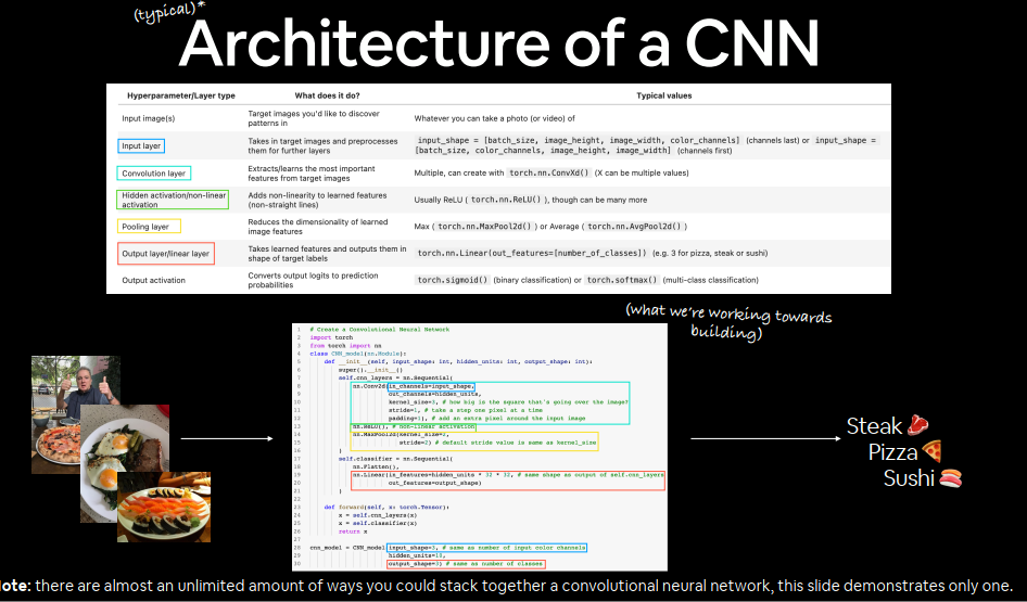
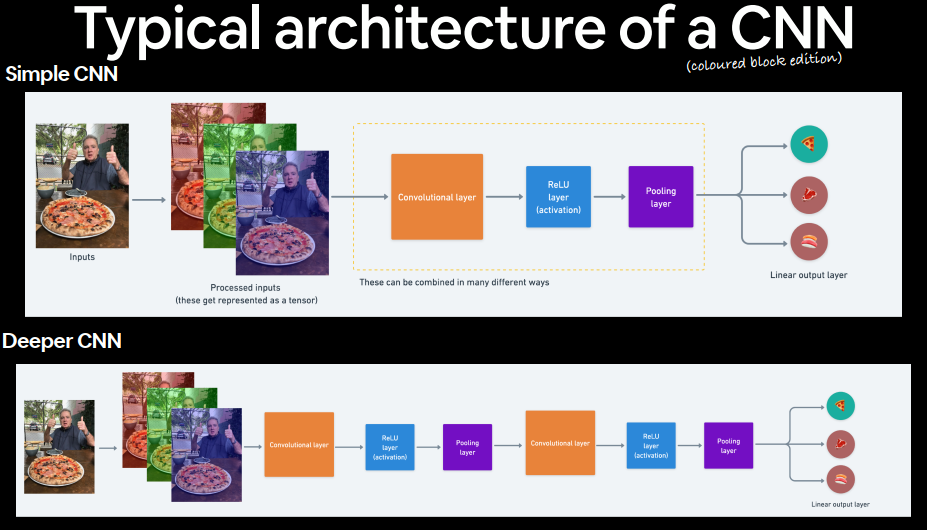
它遵循卷积神经网络的典型结构:
Input layer -> [Convolutional layer -> activation layer -> pooling layer] -> Output layer
根据需要,其中的内容[Convolutional layer -> activation layer -> pooling layer]可以放大和重复多次。
关于模型的讨论已经足够了,现在让我们构建一个 CNN 来复制CNN Explainer 网站 上的模型。
为此,我们将利用nn.Conv2d()nn.MaxPool2d()torch.nn。
1
2
3
4
5
6
7
8
9
10
11
12
13
14
15
16
17
18
19
20
21
22
23
24
25
26
27
28
29
30
31
32
33
34
35
36
37
38
39
40
41
42
43
44
45
46
47
48
49
50
51
52
53
class FashionMNISTModelV2 (nn.Module): """ Model architecture copying TinyVGG from: https://poloclub.github.io/cnn-explainer/ """ def __init__ (self, input_shape: int , hidden_units: int , output_shape: int ): super ().__init__() self.block_1 = nn.Sequential( nn.Conv2d(in_channels=input_shape, out_channels=hidden_units, kernel_size=3 , stride=1 , padding=1 ), nn.ReLU(), nn.Conv2d(in_channels=hidden_units, out_channels=hidden_units, kernel_size=3 , stride=1 , padding=1 ), nn.ReLU(), nn.MaxPool2d(kernel_size=2 , stride=2 ) ) self.block_2 = nn.Sequential( nn.Conv2d(hidden_units, hidden_units, 3 , padding=1 ), nn.ReLU(), nn.Conv2d(hidden_units, hidden_units, 3 , padding=1 ), nn.ReLU(), nn.MaxPool2d(2 ) ) self.classifier = nn.Sequential( nn.Flatten(), nn.Linear(in_features=hidden_units*7 *7 , out_features=output_shape) ) def forward (self, x: torch.Tensor ): x = self.block_1(x) x = self.block_2(x) x = self.classifier(x) return x torch.manual_seed(42 ) model_2 = FashionMNISTModelV2(input_shape=1 , hidden_units=10 , output_shape=len (class_names)).to(device) model_2
1
2
3
4
5
6
7
8
9
10
11
12
13
14
15
16
17
18
19
20
FashionMNISTModelV2( (block_1): Sequential( (0): Conv2d(1, 10, kernel_size=(3, 3), stride=(1, 1), padding=(1, 1)) (1): ReLU() (2): Conv2d(10, 10, kernel_size=(3, 3), stride=(1, 1), padding=(1, 1)) (3): ReLU() (4): MaxPool2d(kernel_size=2, stride=2, padding=0, dilation=1, ceil_mode=False) ) (block_2): Sequential( (0): Conv2d(10, 10, kernel_size=(3, 3), stride=(1, 1), padding=(1, 1)) (1): ReLU() (2): Conv2d(10, 10, kernel_size=(3, 3), stride=(1, 1), padding=(1, 1)) (3): ReLU() (4): MaxPool2d(kernel_size=2, stride=2, padding=0, dilation=1, ceil_mode=False) ) (classifier): Sequential( (0): Flatten(start_dim=1, end_dim=-1) (1): Linear(in_features=490, out_features=10, bias=True) ) )
nn.Conv2d()我们可以开始使用上面的模型,看看会发生什么,但让我们首先逐步了解我们添加的两个新层:
问题:nn.Conv2d()中的“2d”代表什么?
为了测试这些层,让我们创建一些玩具数据,就像 CNN Explainer 上使用的数据一样。
1 2 3 4 5 6 7 8 torch.manual_seed(42 ) images = torch.randn(size=(32 , 3 , 64 , 64 )) test_image = images[0 ] print (f"Image batch shape: {images.shape} -> [batch_size, color_channels, height, width]" )print (f"Single image shape: {test_image.shape} -> [color_channels, height, width]" ) print (f"Single image pixel values:\n{test_image} " )
1
2
3
4
Image batch shape: torch.Size([32, 3, 64, 64]) -> [batch_size, color_channels, height, width] Single image shape: torch.Size([3, 64, 64]) -> [color_channels, height, width] Single image pixel values: tensor([[[ 1.9269, 1.4873, 0.9007, ..., 1.8446, -1.1845, 1.3835],...)
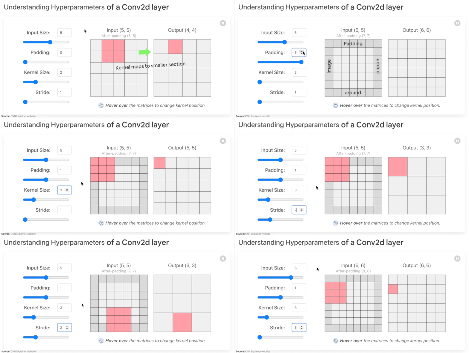
让我们创建一个nn.Conv2d()具有各种参数的示例:
in_channels(int), 输入图像中的通道数。out_channels(int),卷积产生的通道数。kernel_size(int or tuple),卷积核/过滤器的大小。stride(int or tuple, optional),卷积核每次采取的步长。默认值:1。padding(int, tuple, str),在输入的四边添加填充。默认值:0。
更改某nn.Conv2d()一层的超参数时发生的情况的示例。
1 2 3 4 5 6 7 8 9 10 11 12 torch.manual_seed(42 ) conv_layer = nn.Conv2d(in_channels=3 , out_channels=10 , kernel_size=3 , stride=1 , padding=0 ) conv_layer(test_image)
如果尝试传入单张图像,我们会收到形状不匹配错误:
RuntimeError: Expected 4-dimensional input for 4-dimensional weight [10, 3, 3, 3], but got 3-dimensional input of size [3, 64, 64] instead
这是因为我们的nn.Conv2d()层需要一个大小为 (N, C, H, W) 或 [batch_size, color_channels, height, width] 的4 维张量作为输入。
目前我们的单幅图像 test_image 只有 [color_channels, height, width] 或 [3, 64, 64] 的形状。
我们可以使用 test_image.unsqueeze(dim=0) 为单个图像修复此问题,为 N 添加额外的维度。
1 2 test_image.unsqueeze(dim=0 ).shape
1 torch.Size([1, 3, 64, 64])
1 2 conv_layer(test_image.unsqueeze(dim=0 )).shape
1 torch.Size([1, 10, 62, 62])
嗯,注意我们的形状发生了什么变化(与CNN Explainer 上 TinyVGG 的第一层形状相同),我们得到了不同的通道大小以及不同的像素大小。
如果我们改变 conv_layer 的值会怎样?
1 2 3 4 5 6 7 8 9 10 torch.manual_seed(42 ) conv_layer_2 = nn.Conv2d(in_channels=3 , out_channels=10 , kernel_size=(5 , 5 ), stride=2 , padding=0 ) conv_layer_2(test_image.unsqueeze(dim=0 )).shape
1 torch.Size([1, 10, 30, 30])
哇,我们的形状又发生了变化。
现在我们的图像是形状[1, 10, 30, 30](如果使用不同的值,它会有所不同)或[batch_size=1, color_channels=10, height=30, width=30]。
这里发生了什么事?
在幕后,我们nn.Conv2d()正在压缩图像中存储的信息。
它通过根据其内部参数对输入(我们的测试图像)执行操作来实现这一点。
其目标与我们一直在构建的所有其他神经网络类似。
数据输入后,各层会在优化器的帮助下尝试更新其内部参数(模式)以降低损失函数。
唯一的区别在于不同层如何计算它们的参数更新,或者用 PyTorch 术语来说,层方法中存在的操作forward()。
如果我们检查一下,conv_layer_2.state_dict()我们会发现与我们之前看到的类似的权重和偏差设置。
1
2
print (conv_layer_2.state_dict())
权重和偏差张量的一堆随机数。
nn.Conv2d()它们的形状由我们在设置时传递的输入来操纵。
1
2
3
print (f"conv_layer_2 weight shape: \n{conv_layer_2.weight.shape} -> [out_channels=10, in_channels=3, kernel_size=5, kernel_size=5]" )print (f"\nconv_layer_2 bias shape: \n{conv_layer_2.bias.shape} -> [out_channels=10]" )
1
2
3
4
5
conv_layer_2 weight shape: torch.Size([10, 3, 5, 5]) -> [out_channels=10, in_channels=3, kernel_size=5, kernel_size=5] conv_layer_2 bias shape: torch.Size([10]) -> [out_channels=10]
问题:我们应该如何设置图层的参数nn.Conv2d()?
但前提保持不变:从随机数开始并更新它们以更好地表示数据。
nn.MaxPool2d()让我们检查一下当我们移动nn.MaxPool2d()数据时会发生什么。
1
2
3
4
5
6
7
8
9
10
11
12
13
14
print (f"Test image original shape: {test_image.shape} " )print (f"Test image with unsqueezed dimension: {test_image.unsqueeze(dim=0 ).shape} " )max_pool_layer = nn.MaxPool2d(kernel_size=2 ) test_image_through_conv = conv_layer(test_image.unsqueeze(dim=0 )) print (f"Shape after going through conv_layer(): {test_image_through_conv.shape} " )test_image_through_conv_and_max_pool = max_pool_layer(test_image_through_conv) print (f"Shape after going through conv_layer() and max_pool_layer(): {test_image_through_conv_and_max_pool.shape} " )
1
2
3
4
Test image original shape: torch.Size([3, 64, 64]) Test image with unsqueezed dimension: torch.Size([1, 3, 64, 64]) Shape after going through conv_layer(): torch.Size([1, 10, 62, 62]) Shape after going through conv_layer() and max_pool_layer(): torch.Size([1, 10, 31, 31])
注意层内和层外发生的形状的变化nn.MaxPool2d()。
kernel_size层的将nn.MaxPool2d()影响输出形状的大小。
在我们的例子中,形状从一幅62x62图像分成另31x31一幅图像。
让我们用较小的张量看一下这个工作。
1 2 3 4 5 6 7 8 9 10 11 12 13 torch.manual_seed(42 ) random_tensor = torch.randn(size=(1 , 1 , 2 , 2 )) print (f"Random tensor:\n{random_tensor} " )print (f"Random tensor shape: {random_tensor.shape} " )max_pool_layer = nn.MaxPool2d(kernel_size=2 ) max_pool_tensor = max_pool_layer(random_tensor) print (f"\nMax pool tensor:\n{max_pool_tensor} <- this is the maximum value from random_tensor" )print (f"Max pool tensor shape: {max_pool_tensor.shape} " )
1
2
3
4
5
6
7
8
Random tensor: tensor([[[[0.3367, 0.1288], [0.2345, 0.2303]]]]) Random tensor shape: torch.Size([1, 1, 2, 2]) Max pool tensor: tensor([[[[0.3367]]]]) <- this is the maximum value from random_tensor Max pool tensor shape: torch.Size([1, 1, 1, 1])
注意 random_tensor 和 max_pool_tensor 之间的最后两个维度,它们从 [2, 2] 变为 [1, 1]。nn.MaxPool2d(),kernel_size 的不同值,变化会有所不同。max_pool_tensor 中剩余的值是 random_tensor 中的最大值。
这里发生了什么事?神经网络中的每一层都试图将数据从高维空间压缩到低维空间。
从人工智能的角度来看,你可以将神经网络的整个目标视为压缩信息。
这意味着,从神经网络的角度来看,智能就是压缩。
这是使用nn.MaxPool2d()层的想法:从张量的一部分中取最大值,而忽略其余部分。
本质上,降低张量的维数,同时仍然保留(希望)很大一部分信息。
对于层来说也是同样的情况nn.Conv2d()。
除了不只是取最大值之外,还对数据执行卷积运算(请参阅CNN 解释器网页 nn.Conv2d()上的实际操作)。
练习: 您认为该nn.AvgPool2d()课外活动: 查找“最常见的卷积神经网络”,你找到了哪些架构?库中包含其中的任何架构吗torchvision.models
model_2我们将像以前一样使用这些函数,nn.CrossEntropyLoss() 作为损失函数(因为我们处理的是多类分类数据)。
并使用 torch.optim.SGD() 作为优化器,以 0.1 的学习率优化 model_2.parameters()。
1
2
3
4
loss_fn = nn.CrossEntropyLoss() optimizer = torch.optim.SGD(params=model_2.parameters(), lr=0.1 )
model_2 using our training and test functions损失和优化器已准备好!训练和测试的时间。train_step()和test_step()函数。
1 2 3 4 5 6 7 8 9 10 11 12 13 14 15 16 17 18 19 20 21 22 23 24 25 26 27 28 torch.manual_seed(42 ) from timeit import default_timer as timertrain_time_start_model_2 = timer() epochs = 3 for epoch in tqdm(range (epochs)): print (f"Epoch: {epoch} \n---------" ) train_step(data_loader=train_dataloader, model=model_2, loss_fn=loss_fn, optimizer=optimizer, accuracy_fn=accuracy_fn, device=device ) test_step(data_loader=test_dataloader, model=model_2, loss_fn=loss_fn, accuracy_fn=accuracy_fn, device=device ) train_time_end_model_2 = timer() total_train_time_model_2 = print_train_time(start=train_time_start_model_2, end=train_time_end_model_2, device=device)
1
2
3
4
5
6
7
8
9
10
11
12
13
14
15
16
Epoch: 0 --------- Train loss: 0.59664 | Train accuracy: 78.43% Test loss: 0.38824 | Test accuracy: 86.24% Epoch: 1 --------- Train loss: 0.35712 | Train accuracy: 87.12% Test loss: 0.34803 | Test accuracy: 87.15% Epoch: 2 --------- Train loss: 0.31907 | Train accuracy: 88.50% Test loss: 0.32589 | Test accuracy: 88.37% Train time on cuda: 51.457 seconds
看起来卷积层和最大池化层有助于提高性能。
让我们model_2用我们的函数评估的结果eval_model()。
1
2
3
4
5
6
7
8
model_2_results = eval_model( model=model_2, data_loader=test_dataloader, loss_fn=loss_fn, accuracy_fn=accuracy_fn ) model_2_results
1
2
3
{'model_name': 'FashionMNISTModelV2', 'model_loss': 0.3258868157863617, 'model_acc': 88.36861022364218}
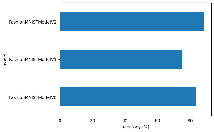
我们训练了三种不同的模型。
model_0,我们的基线模型有两层nn.Linear()。model_1,与我们的基线模型设置相同,只是层与层nn.ReLU()之间有层nn.Linear()。model_2,我们的第一个 CNN 模型模仿了 CNN Explainer 网站上的 TinyVGG 架构。
这是机器学习的常规做法。
建立多个模型并进行多次训练实验,以查看哪个表现最佳。
让我们将模型结果字典合并到 DataFrame 中并找出答案。
1
2
3
import pandas as pdcompare_results = pd.DataFrame([model_0_results, model_1_results, model_2_results]) compare_results
model_name
model_loss
model_acc
FashionMNISTModelV0
0.476639
83.426518
FashionMNISTModelV1
0.685001
75.019968
FashionMNISTModelV2
0.325887
88.368610
添加训练时间值。
1 2 3 4 5 compare_results["training_time" ] = [total_train_time_model_0, total_train_time_model_1, total_train_time_model_2] compare_results
model_name
model_loss
model_acc
training_time
FashionMNISTModelV0
0.476639
83.426518
463.021015
FashionMNISTModelV1
0.685001
75.019968
45.538106
FashionMNISTModelV2
0.325887
88.368610
52.672458
看起来我们的 CNN(FashionMNISTModelV2)模型表现最佳(损失最低、准确度最高),但训练时间最长。
并且我们的基线模型 ( FashionMNISTModelV0) 的表现优于model_1( FashionMNISTModelV1)。
在机器学习中需要注意的是性能和速度的权衡。
一般来说,更大、更复杂的模型会获得更好的性能(就像我们所做的那样model_2)。
然而,这种性能的提升往往是以牺牲训练速度和推理速度为代价的。
1 2 3 4 compare_results.set_index("model_name" )["model_acc" ].plot(kind="barh" ) plt.xlabel("accuracy (%)" ) plt.ylabel("model" );
将我们的模型相互比较了,让我们进一步评估我们表现最好的模型model_2。
为此,让我们创建一个函数make_predictions(),我们可以在其中传递模型和一些数据以供其预测。
1
2
3
4
5
6
7
8
9
10
11
12
13
14
15
16
17
18
19
def make_predictions (model: torch.nn.Module, data: list , device: torch.device = device ): pred_probs = [] model.eval () with torch.inference_mode(): for sample in data: sample = torch.unsqueeze(sample, dim=0 ).to(device) pred_logit = model(sample) pred_prob = torch.softmax(pred_logit.squeeze(), dim=0 ) pred_probs.append(pred_prob.cpu()) return torch.stack(pred_probs)
1
2
3
4
5
6
7
8
9
10
import randomrandom.seed(42 ) test_samples = [] test_labels = [] for sample, label in random.sample(list (test_data), k=9 ): test_samples.append(sample) test_labels.append(label) print (f"Test sample image shape: {test_samples[0 ].shape} \nTest sample label: {test_labels[0 ]} ({class_names[test_labels[0 ]]} )" )
1
2
Test sample image shape: torch.Size([1, 28, 28]) Test sample label: 5 (Sandal)
现在我们可以使用 make_predictions() 函数来预测 test_samples。
1
2
3
4
5
6
pred_probs= make_predictions(model=model_2, data=test_samples) pred_probs[:2 ]
1
2
3
4
tensor([[7.7393e-08, 6.9452e-08, 7.9230e-09, 7.5061e-08, 1.0008e-08, 9.9992e-01, 1.6065e-06, 6.7758e-07, 6.3521e-06, 7.4828e-05], [2.0884e-02, 8.1752e-01, 6.5737e-04, 6.4430e-02, 6.4946e-02, 4.4571e-04, 2.9005e-02, 2.8220e-04, 7.9620e-04, 1.0312e-03]])
现在,我们可以通过获取 torch.softmax() 激活函数输出的 torch.argmax() 从预测概率转到预测标签。
1
2
3
pred_classes = pred_probs.argmax(dim=1 ) pred_classes
1 tensor([5, 1, 7, 4, 3, 0, 4, 7, 1])
1
2
test_labels, pred_classes
1 ([5, 1, 7, 4, 3, 0, 4, 7, 1], tensor([5, 1, 7, 4, 3, 0, 4, 7, 1]))
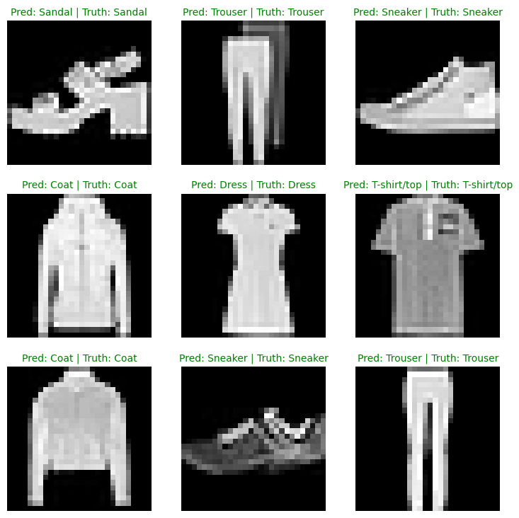
现在,我们预测的类别与测试标签的格式相同,我们可以进行比较了。
1 2 3 4 5 6 7 8 9 10 11 12 13 14 15 16 17 18 19 20 21 22 23 24 25 26 plt.figure(figsize=(9 , 9 )) nrows = 3 ncols = 3 for i, sample in enumerate (test_samples): plt.subplot(nrows, ncols, i+1 ) plt.imshow(sample.squeeze(), cmap="gray" ) pred_label = class_names[pred_classes[i]] truth_label = class_names[test_labels[i]] title_text = f"Pred: {pred_label} | Truth: {truth_label} " if pred_label == truth_label: plt.title(title_text, fontsize=10 , c="g" ) else : plt.title(title_text, fontsize=10 , c="r" ) plt.axis(False );
对于分类问题,我们可以使用许多不同的评估指标。
最直观的一种是混淆矩阵 。
混淆矩阵可以显示分类模型在预测和真实标签之间混淆的地方。
为了制作混淆矩阵,我们将经历三个步骤:model_2(混淆矩阵将预测与真实标签进行比较)。torchmetrics.ConfusionMatrix。mlxtend.plotting.plot_confusion_matrix()。
1
2
3
4
5
6
7
8
9
10
11
12
13
14
15
16
17
18
from tqdm.auto import tqdmy_preds = [] model_2.eval () with torch.inference_mode(): for X, y in tqdm(test_dataloader, desc="Making predictions" ): X, y = X.to(device), y.to(device) y_logit = model_2(X) y_pred = torch.softmax(y_logit, dim=1 ).argmax(dim=1 ) y_preds.append(y_pred.cpu()) y_pred_tensor = torch.cat(y_preds)
1
2
3
4
5
6
7
8
9
try : import torchmetrics, mlxtend print (f"mlxtend version: {mlxtend.__version__} " ) assert int (mlxtend.__version__.split("." )[1 ]) >= 19 , "mlxtend verison should be 0.19.0 or higher" except : !pip install -q torchmetrics -U mlxtend import torchmetrics, mlxtend print (f"mlxtend version: {mlxtend.__version__} " )
1
2
3
4
import mlxtend print (mlxtend.__version__)assert int (mlxtend.__version__.split("." )[1 ]) >= 19
torchmetrics 和 mlxtend安装完毕,让我们制作一个混淆矩阵!
首先,我们将创建一个torchmetrics.ConfusionMatrix实例,通过设置来告诉它我们要处理多少个类num_classes=len(class_names)。
然后,我们将通过向我们的实例传递模型的预测(preds=y_pred_tensor)和目标(target=test_data.targets)来创建一个混淆矩阵(张量格式)。
plot_confusion_matrix()最后,我们可以使用中的函数绘制混淆矩阵mlxtend.plotting。
1
2
3
4
5
6
7
8
9
10
11
12
13
14
from torchmetrics import ConfusionMatrixfrom mlxtend.plotting import plot_confusion_matrixconfmat = ConfusionMatrix(num_classes=len (class_names), task='multiclass' ) confmat_tensor = confmat(preds=y_pred_tensor, target=test_data.targets) fig, ax = plot_confusion_matrix( conf_mat=confmat_tensor.numpy(), class_names=class_names, figsize=(10 , 7 ) );
哇哦!看起来不是很棒吗?
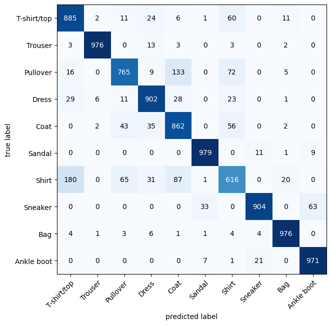
我们可以看到我们的模型表现相当好,因为大多数深色方块都位于从左上到右下的对角线上(理想模型只有在这些方块中有值,其他地方都为 0)。
该模型对相似的类别最为“困惑”,例如,对于实际标记为“衬衫”的图像,预测其为“套头衫”。
对于实际标记为“T 恤/上衣”的类别,预测其为“衬衫”,方法也是一样。
这种信息通常比单一的准确度指标更有帮助,因为它可以告诉我们模型哪里出了问题。
它也暗示了为什么模型可能会出现某些错误。
可以理解的是,对于标有“T 恤/上衣”的图像,模型有时会预测“衬衫”。
我们可以利用此类信息进一步检查我们的模型和数据,看看如何改进。
使用以下组合来保存和加载 PyTorch 模型:
torch.save- 用于保存整个 PyTorch 模型或模型的函数state_dict()。torch.load- 用于加载已保存的 PyTorch 对象的函数。torch.nn.Module.load_state_dict()- 将保存的state_dict()内容加载到现有模型实例中的功能。
保存 model_2 的 state_dict() 然后重新加载并评估它,以确保 保存 和 加载 正确进行。
1
2
3
4
5
6
7
8
9
10
11
12
13
14
15
16
from pathlib import PathMODEL_PATH = Path("models" ) MODEL_PATH.mkdir(parents=True , exist_ok=True ) MODEL_NAME = "03_pytorch_computer_vision_model_2.pth" MODEL_SAVE_PATH = MODEL_PATH / MODEL_NAME print (f"Saving model to: {MODEL_SAVE_PATH} " )torch.save(obj=model_2.state_dict(), f=MODEL_SAVE_PATH)
1 Saving model to: models/03_pytorch_computer_vision_model_2.pth
现在我们已经有一个保存的模型,我们可以使用和的state_dict()组合将其重新加载。load_state_dict()torch.load()
由于我们正在使用load_state_dict(),我们需要创建一个FashionMNISTModelV2()具有与我们保存的模型相同的输入参数的新实例state_dict()。
1
2
3
4
5
6
7
8
9
10
11
loaded_model_2 = FashionMNISTModelV2(input_shape=1 , hidden_units=10 , output_shape=10 ) loaded_model_2.load_state_dict(torch.load(f=MODEL_SAVE_PATH)) loaded_model_2 = loaded_model_2.to(device)
现在我们已经有一个加载的模型,我们可以对其进行评估,eval_model()以确保其参数与model_2保存之前的工作方式类似。
1 2 3 4 5 6 7 8 9 10 11 torch.manual_seed(42 ) loaded_model_2_results = eval_model( model=loaded_model_2, data_loader=test_dataloader, loss_fn=loss_fn, accuracy_fn=accuracy_fn ) loaded_model_2_results
1
2
3
{'model_name': 'FashionMNISTModelV2', 'model_loss': 0.3258868157863617, 'model_acc': 88.36861022364218}
这些结果看起来是否相同model_2_results?
1
2
3
{'model_name': 'FashionMNISTModelV2', 'model_loss': 0.3258868157863617, 'model_acc': 88.36861022364218}
我们可以使用 torch.isclose() 来确定两个张量是否彼此接近,并通过参数 atol(绝对容差)和 rtol(相对容差)传入接近度的容差级别。
如果我们的模型的结果接近,则 torch.isclose() 的输出应该为 true。
1 2 3 4 5 torch.isclose(torch.tensor(model_2_results["model_loss" ]), torch.tensor(loaded_model_2_results["model_loss" ]), atol=1e-08 , rtol=0.0001 )
所有练习都集中于练习以上部分中的代码。
您应该能够通过参考每个部分或按照链接的资源来完成它们。
所有练习都应使用与设备无关的代码 来完成。
资源:
目前计算机视觉在工业领域中的应用有哪三个?
搜索“机器学习中的过度拟合是什么”,然后写下你发现的内容。
搜索“机器学习中防止过度拟合的方法”,写下你发现的 3 件事,并写下每件事的一句话。注意: 有很多这样的方法,所以不要太担心所有方法,只需选择 3 个并从中开始。
花 20 分钟阅读和点击 CNN Explainer 网站
使用“上传”按钮上传您自己的示例图像,并查看当您的图像通过 CNN 时其每一层发生的情况。
加载torchvision.datasets.MNIST()
可视化 MNIST 训练数据集的至少 5 个不同样本。
将 MNIST 训练和测试数据集转换为数据加载器torch.utils.data.DataLoader,设置batch_size=32。
重新创建在此笔记本中使用的模型(来自CNN Explainer 网站 model_2的相同模型,也称为 TinyVGG),能够适合 MNIST 数据集。
在 CPU 和 GPU 上训练你在练习 8 中构建的模型,并查看每个模型需要多长时间。
使用训练好的模型进行预测,并将其中至少 5 个预测与目标标签进行比较。
绘制混淆矩阵,将模型的预测与真实标签进行比较。
创建一个形状的随机张量[1, 3, 64, 64],并将其传递到具有各种超参数设置的层(这些可以是您选择的任何设置),如果参数上升和下降,nn.Conv2d()您会注意到什么?kernel_size
model_2使用与本笔记本训练的模型类似的模型对测试torchvision.datasets.FashionMNIST 数据集进行预测。
然后绘制一些模型错误的预测以及图像的标签应该是什么。
在将这些预测可视化之后,您认为这更多的是建模错误还是数据错误?
例如,模型是否可以做得更好,或者数据的标签是否太接近(例如,“衬衫”标签太接近“T 恤/上衣”)?