PyTorch-26H-3

主页：https://www.freecodecamp.org/news/learn-pytorch-for-deep-learning-in-day/

github：https://github.com/mrdbourke/pytorch-deep-learning

Learn PyTorch for Deep Learning: Zero to Mastery book：https://www.learnpytorch.io/

PyTorch documentation：https://pytorch.org/docs/stable/index.html

What is a classification problem? 什么是分类问题？

问题类型	解释	例子
二元分类(Binary classification)	目标可以是两个选项之一，例如是或否	根据某人的健康参数预测他是否患有心脏病。
多类别分类(Multi-class classification)	目标可以是两个以上选项之一	确定照片中是食物、人还是狗。
多标签分类(Multi-label classification)	目标可以分配多个选项	预测应为维基百科文章分配哪些类别（例如数学、科学和哲学）。

PyTorch-26H-3-1 PyTorch-26H-3-2

分类和回归是最常见的机器学习问题类型之一。

换句话说，获取一组输入并预测该组输入属于哪个类别。

What we’re going to cover 我们将要讨论的内容

Architecture of a neural network classification model
神经网络分类模型的架构
Input shapes and output shapes of a classification model (features and labels)
分类模型的输入形状和输出形状（特征和标签）
Creating custom data to view, fit on and predict on
创建自定义数据以查看、拟合和预测
Steps in modelling
建模步骤
Creating a model, setting a loss function and optimiser, creating a training loop, evaluating a
model
创建模型、设置损失函数和优化器、创建训练循环、评估
Saving and loading models
保存和加载模型
Harnessing the power of non-linearity
利用非线性的力量
Different classification evaluation methods
不同的分类评估方法

话题	内容
0. 分类神经网络的架构	神经网络几乎可以具有任何形状和大小，但它们通常遵循类似的平面图。
1. 准备二元分类数据	数据几乎可以是任何东西，但首先我们将创建一个简单的二元分类数据集。
2.构建 PyTorch 分类模型	在这里我们将创建一个模型来学习数据中的模式，我们还将选择一个损失函数、优化器并构建一个特定于分类的训练循环。
3. 将模型拟合到数据（训练）	我们有数据和模型，现在让我们让模型（尝试）在（训练）数据中寻找模式。
4. 做出预测并评估模型（推理）	我们的模型在数据中发现了模式，让我们将它的发现与实际（测试）数据进行比较。
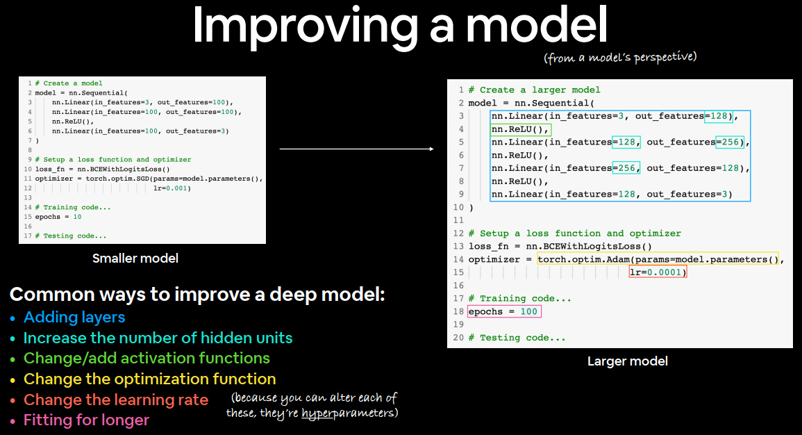
5. 改进模型（从模型角度）	我们已经训练并评估了一个模型，但它不起作用，让我们尝试一些方法来改进它。
6.非线性	到目前为止，我们的模型只具有对直线进行建模的能力，那么非线性（非直线）线又如何呢？
7. 复制非线性函数	我们使用非线性函数来帮助建模非线性数据，但是这些函数是什么样子的？
8. 将所有内容与多类别分类结合起来	让我们将迄今为止为二元分类所做的一切与多类分类问题放在一起。

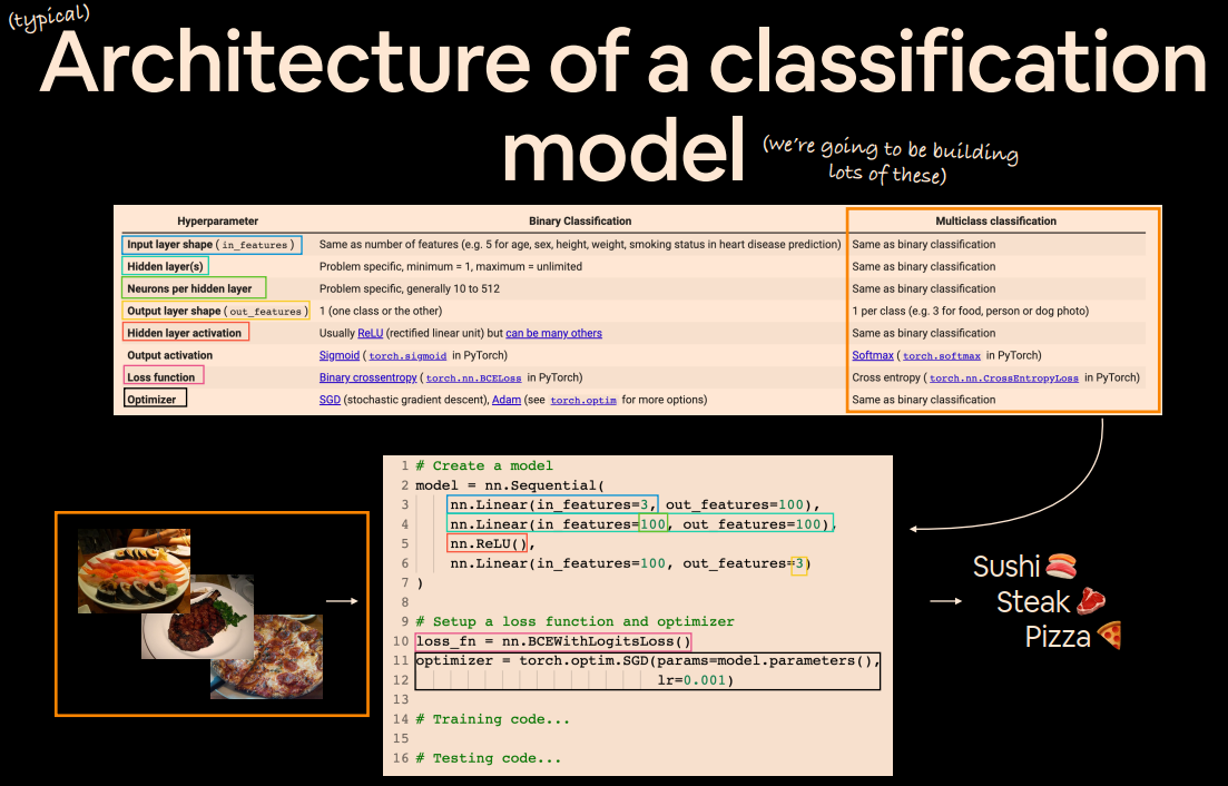
0. Architecture of a classification neural network 分类神经网络的架构

分类神经网络的一般架构：

这个分类神经网络组件的成分列表会根据您正在处理的问题而有所不同。

PyTorch-26H-3-2_1

1. Make classification data and get it ready 分类数据制作及准备

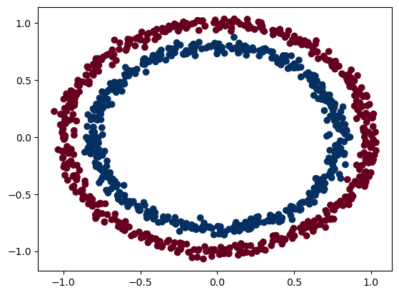
使用 make_circles() 中的 Scikit-Learn 方法生成两个具有不同颜色的圆圈。


from sklearn.datasets import make_circles


n_samples = 1000


X, y = make_circles(n_samples,
                    noise = 0.03, 
                    random_state = 42)

查看前5个X值y。

1 2	print(f"First 5 X features:\n{X[:5]}") print(f"\nFirst 5 y labels:\n{y[:5]}")

First 5 X features:
[[ 0.75424625  0.23148074]
 [-0.75615888  0.15325888]
 [-0.81539193  0.17328203]
 [-0.39373073  0.69288277]
 [ 0.44220765 -0.89672343]]

First 5 y labels:
[1 1 1 1 0]

可视化：


import pandas as pd
circles = pd.DataFrame({"X1": X[:, 0],
    				   "X2": X[:, 1],
    				   "label": y})
circles.head(10)

	X1	X2	label
0	0.754246	0.231481	1
1	-0.756159	0.153259	1
2	-0.815392	0.173282	1
3	-0.393731	0.692883	1
4	0.442208	-0.896723	0
5	-0.479646	0.676435	1
6	-0.013648	0.803349	1
7	0.771513	0.147760	1
8	-0.169322	-0.793456	1
9	-0.121486	1.021509	0

看起来每对X特征（X1和X2）都有一个标签（y）值，即 0 或 1。

这告诉我们我们的问题是二元分类，因为只有两个选项（0 或 1）。

每个类别有多少个值？

1 2	circles.label.value_counts()

1
2
3

1    500
0    500
Name: label, dtype: int64

0和1各五百个


import matplotlib.pyplot as plt
plt.scatter(x=X[:, 0], 
            y=X[:, 1], 
            c=y, 
            cmap=plt.cm.RdYlBu);

PyTorch-26H-3-3

如何构建 PyTorch 神经网络来将点分类为红色（0）或蓝色（1）。

在机器学习中，这个数据集通常被视为玩具问题（用于尝试和测试事物的问题）。但它代表了分类的主要关键，您有一些以数值表示的数据，并且您想要构建一个能够对其进行分类的模型，在我们的例子中，将其分成红点或蓝点。

scikit-learn-toy datasets

1.1 Input and output shapes 输入和输出形状

PyTorch-26H-3-3_1 PyTorch-26H-3-3_2

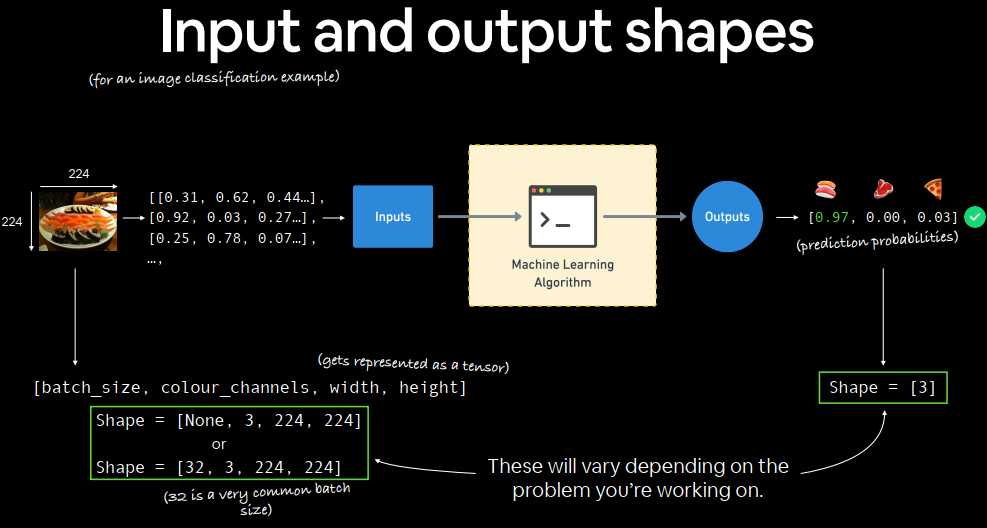
可以设置32的batch size。使用大型 minibatch 进行训练对测试错误不利。

深度学习中最常见的错误之一是形状错误。

张量形状和张量运算不匹配将导致模型出现错误。

我们将会在整个课程中看到很多这样的情况。

输入和输出形状。

1 2	X.shape, y.shape

1	((1000, 2), (1000,))

看起来我们在每个维度的第一维度上都找到了匹配项。

有 1000 个 X 和 1000 个 y。

但是 X 的第二维度是什么？

查看单个样本（特征和标签）的值和形状通常很有帮助。

这样做将帮助您了解您希望从模型中获得什么样的输入和输出形状。


X_sample = X[0]
y_sample = y[0]
print(f"Values for one sample of X: {X_sample} and the same for y: {y_sample}")
print(f"Shapes for one sample of X: {X_sample.shape} and the same for y: {y_sample.shape}")

1 2	Values for one sample of X: [0.75424625 0.23148074] and the same for y: 1 Shapes for one sample of X: (2,) and the same for y: ()

这告诉我们 X 的第二个维度意味着它有两个特征（向量vector），而 y 只有一个特征（标量scalar）。

我们有两个输入和一个输出。

1.2 Turn data into tensors and create train and test splits 将数据转换为张量并创建训练和测试分割

1、将我们的数据转换成张量（现在我们的数据在 NumPy 数组中，PyTorch 更喜欢使用 PyTorch 张量）。
2、X将我们的数据分成训练集和测试集（我们将在训练集上训练一个模型来学习和之间的模式，y然后在测试数据集上评估这些学习到的模式）。



import torch
X = torch.from_numpy(X).type(torch.float)
y = torch.from_numpy(y).type(torch.float)


X[:5], y[:5]

(tensor([[ 0.7542,  0.2315],
         [-0.7562,  0.1533],
         [-0.8154,  0.1733],
         [-0.3937,  0.6929],
         [ 0.4422, -0.8967]]),
 tensor([1., 1., 1., 1., 0.]))

1	type(X), X.dtype, y.dtype

1	(torch.Tensor, torch.float32, torch.float32)

现在我们的数据是张量格式，让我们将其分成训练集和测试集。

使用 Scikit-Learn 中 train_test_split() 函数。

我们将使用test_size=0.2（80％训练，20％测试），并且由于分割在数据中随机发生，random_state=42因此我们使用可重现的分割。


from sklearn.model_selection import train_test_split

X_train, X_test, y_train, y_test = train_test_split(X, 
                            y, 
                            test_size=0.2, 
                            random_state=42) 

len(X_train), len(X_test), len(y_train), len(y_test)

1	(800, 200, 800, 200)

现在有 800 个训练样本和 200 个测试样本。

2. Building a model 建立模型

模型需要分为几个部分。

1、设置与设备无关的代码（这样我们的模型可以在 CPU 或 GPU 上运行）。
2、通过子类化构建模型 nn.Module。
3、定义损失函数和优化器。
4、创建训练循环。

设置与设备无关的代码


import torch
from torch import nn


device = "cuda" if torch.cuda.is_available() else "cpu"
device

'cuda'

通过子类化构建模型

我们需要一个模型，能够处理我们的X数据作为输入，并生成与我们的数据形状相同y的输出。

换句话说，给定X（特征feature），我们希望我们的模型预测y（标签label）。

这种具有特征和标签的设置称为监督学习。因为你的数据会告诉你的模型，给定某个输入，应该得到什么样的输出。

要创建这样的模型，需要处理X和的输入和输出形状y。

创建一个模型类：

1、子类 nn.Module（几乎所有 PyTorch 模型都是 nn.Module 的子类）。
2、在构造函数中创建 2 个 nn.Linear 层，能够处理 X 和 y 的输入和输出形状。
3、定义一个包含模型前向传递计算的 forward() 方法。
4、实例化模型类并将其发送到目标设备。


class CircleModelV0(nn.Module):
    def __init__(self):
        super().__init__()
        
        self.layer_1 = nn.Linear(in_features=2, out_features=5) 
        self.layer_2 = nn.Linear(in_features=5, out_features=1) 

    
    def forward(self, x):
        
        return self.layer_2(self.layer_1(x)) 
    	


model_0 = CircleModelV0().to(device)
model_0

CircleModelV0(
  (layer_1): Linear(in_features=2, out_features=5, bias=True)
  (layer_2): Linear(in_features=5, out_features=1, bias=True)
)

device

'cuda'

1	next(model_0.parameters()).device

1	device(type='cuda', index=0)

PyTorch-26H-3-3_3

50%的准确率，跟盲猜一样。

唯一的重大变化是 self.layer_1 和 self.layer_2 之间发生的事情。

self.layer_1 接受 2 个输入特征 in_features=2 并产生 5 个输出特征 out_features=5。

这被称为具有 5 个隐藏单元或神经元。该层将输入数据从 2 个特征变为 5 个特征。

这使得模型可以从 5 个数字而不是仅仅 2 个数字中学习模式，从而可能产生更好的输出。

在神经网络层中使用的隐藏单元的数量是一个超参数（可以自己设置的值），并且没有必须使用的固定值。
通常情况下，数量越多越好，但也可能太多。您选择的数量取决于您的模型类型和您正在使用的数据集。

由于我们的数据集很小而且简单，因此我们会将其保持较小。

隐藏单元的唯一规则是下一层（在我们的例子中为 self.layer_2）必须采用与前一层 out_features 相同的 in_features。

这就是为什么 self.layer_2 有 in_features=5，它从 self.layer_1 中获取 out_features=5 并对它们执行线性计算，将它们转换为 out_features=1（与 y 相同的形状）。

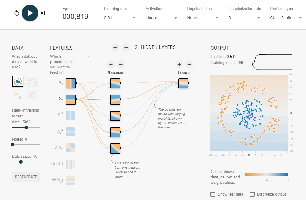
与我们刚刚构建的分类神经网络类似的视觉示例。尝试在 TensorFlow Playground 网站上创建一个您自己的神经网络。

Sequential 和 nn.model的区别

您也可以使用 nn.Sequential 执行与上述相同的操作。


model_0 = nn.Sequential(
    nn.Linear(in_features=2, out_features=5),
    nn.Linear(in_features=5, out_features=1)
).to(device)

model_0

Sequential(
  (0): Linear(in_features=2, out_features=5, bias=True)
  (1): Linear(in_features=5, out_features=1, bias=True)
)

这看起来比子类化简单多了 nn.Module，为什么不总是使用呢nn.Sequential？

nn.Sequential对于直接计算来说非常棒，但是，正如命名空间所说，它总是按顺序运行。

因此，如果您希望发生其他事情（而不仅仅是直接的顺序计算），您将需要定义自己的自定义nn.Module子类。

例如使用Sequential建立的模型，可以融合到nn.model中去

model_0 = nn.Sequential(
    nn.Linear(in_features=2, out_features=5),
    nn.Linear(in_features=5, out_features=1)
).to(device)



class CircleModelV0(nn.Module):
    def __init__(self):
        super().__init__()
        
      	self.two_linear_layer = nn.Sequential(
      		nn.Liner(in_features=2, out_features=5),
      		nn.Liner(in_features=5, out_features=1)
      	)

    def forward(self, x):
      return self.two_linear_layer(x)

1	model_0.state_dict()

OrderedDict([('0.weight',
              tensor([[ 0.2259, -0.3071],
                      [ 0.1391, -0.4125],
                      [ 0.0519, -0.6626],
                      [ 0.0739,  0.2506],
                      [ 0.3370,  0.2946]])),
             ('0.bias', tensor([0.0039, 0.5227, 0.4068, 0.2547, 0.0523])),
             ('1.weight',
              tensor([[ 0.0300, -0.3890,  0.2665,  0.0364,  0.2124]])),
             ('1.bias', tensor([-0.2119]))])

修改模型隐藏层个数会产生不同的state_dict信息

观察模型传递数据

通过模型传递一些数据时会发生什么。


untrained_preds = model_0(X_test.to(device))
print(f"Length of predictions: {len(untrained_preds)}, Shape: {untrained_preds.shape}")
print(f"Length of test samples: {len(y_test)}, Shape: {y_test.shape}")
print(f"\nFirst 10 predictions:\n{untrained_preds[:10]}")
print(f"\nFirst 10 test labels:\n{y_test[:10]}")

Length of predictions: 200, Shape: torch.Size([200, 1])
Length of test samples: 200, Shape: torch.Size([200])

First 10 predictions:
tensor([[-0.1631],
        [-0.4051],
        [ 0.3693],
        [-0.3135],
        [ 0.2072],
        [ 0.0607],
        [-0.4923],
        [-0.3836],
        [ 0.3753],
        [-0.4231]], device='cuda:0', grad_fn=<SliceBackward0>)

First 10 test labels:
tensor([1., 0., 1., 0., 1., 1., 0., 0., 1., 0.])


with torch.inference_mode():
  untrained_preds = model_0(X_test.to(device))
print(f"Length of predictions: {len(untrained_preds)}, Shape: {untrained_preds.shape}")
print(f"Length of test samples: {len(X_test)}, Shape: {X_test.shape}")
print(f"\nFirst 10 predictions:\n{torch.round(untrained_preds[:10])}")
print(f"\nFirst 10 labels:\n{y_test[:10]}")

Length of predictions: 200, Shape: torch.Size([200, 1])
Length of test samples: 200, Shape: torch.Size([200, 2])

First 10 predictions:
tensor([[-0.],
        [-0.],
        [-0.],
        [-0.],
        [0.],
        [0.],
        [-0.],
        [-0.],
        [-0.],
        [-0.]], device='cuda:0')

First 10 labels:
tensor([1., 0., 1., 0., 1., 1., 0., 0., 1., 0.])

预测的数量与测试标签的数量相同，但是预测的形式或形状看起来与测试标签不一样。

定义损失函数和优化器

不同类型的问题需要不同的损失函数。

损失函数衡量模型预测的错误程度。

回归问题（预测数字）：使用平均绝对误差（MAE）损失。
二元分类问题（目前的问题），使用二元交叉熵作为损失函数。

相同的优化器函数通常可用于不同的问题空间。

随机梯度下降优化器（SGD，torch.optim.SGD()）可用于解决一系列问题，Adam 优化器（torch.optim.Adam()）同样适用。

由于我们正在处理二元分类问题，因此我们使用二元交叉熵损失函数。

什么是logit？

logit-wiki
有关损失函数和优化器的一些常见选择
对于损失函数，我们将使用 torch.nn.BECWithLogitsLoss()，有关二元交叉熵 (BCE) 的更多信息，请查看本文
 有关深度学习中 logit 的定义
有关不同的优化器，请参阅 torch.optim

PyTorch 有两种二元交叉熵实现：

1、torch.nn.BCELoss()- 创建一个损失函数，测量目标（标签）和输入（特征）之间的二元交叉熵。
2、torch.nn.BCEWithLogitsLoss() - 这与上面的相同，只是它有一个内置的 sigmoid 层 (nn.Sigmoid)

torch.nn.BCEWithLogitsLoss() 的文档指出，它比在 nn.Sigmoid 层之后使用 torch.nn.BCELoss() 更具数值稳定性。

通常，实现 2 是更好的选择。但是对于高级用法，可能希望分离 nn.Sigmoid 和 torch.nn.BCELoss() 的组合，但这超出了本笔记本的范围。

了解了这一点，让我们创建一个损失函数和一个优化器。

对于优化器，我们将使用 torch.optim.SGD() 以学习率为 0.1 来优化模型参数。



loss_fn = nn.BCEWithLogitsLoss() 


optimizer = torch.optim.SGD(params=model_0.parameters(), 
                            lr=0.1)

1	model_0.state_dict()

OrderedDict([('0.weight',
              tensor([[ 0.2259, -0.3071],
                      [ 0.1391, -0.4125],
                      [ 0.0519, -0.6626],
                      [ 0.0739,  0.2506],
                      [ 0.3370,  0.2946]])),
             ('0.bias', tensor([0.0039, 0.5227, 0.4068, 0.2547, 0.0523])),
             ('1.weight',
              tensor([[ 0.0300, -0.3890,  0.2665,  0.0364,  0.2124]])),
             ('1.bias', tensor([-0.2119]))])

创建一个评估指标

损失函数衡量模型的错误程度 → 评估指标视为衡量模型的正确程度。

评估指标提供了不同的视角。
在评估模型时，最好从多个角度看待事物。
有几种评估指标可用于分类问题，但让我们从准确度开始。
准确度可以通过将正确预测的总数除以预测总数来衡量。
例如，如果一个模型在 100 个预测中做出 99 个正确的预测，则准确度为 99%。


def accuracy_fn(y_true, y_pred):
    correct = torch.eq(y_true, y_pred).sum().item() 
    acc = (correct / len(y_pred)) * 100 
    return acc

现在可以在训练模型时使用此功能来测量其性能和损失。

3. Train model

PyTorch 训练循环步骤：

1、前向传递 Forward pass - 模型对所有训练数据进行一次遍历，执行其 forward() 函数计算 (model(x_train))。
2、计算损失 Calculate the loss - 将模型的输出 (预测) 与基本事实进行比较，并进行评估以查看其错误程度 (loss = loss_fn(y_pred, y_train))。
3、零梯度 Zero gradients - 优化器梯度设置为零 (默认情况下是累积的)，因此可以为特定的训练步骤重新计算 (optimizer.zero_grad())。
4、对损失执行反向传播 Perform backpropagation on the loss - 针对要更新的每个模型参数 (每个参数的 require_grad=True) 计算损失的梯度。这称为反向传播，因此为“向后”(loss.backward())。
5、步进优化器 (梯度下降) Step the optimizer (gradient descent) - 使用 require_grad=True 更新参数，以根据损失梯度改进它们 (optimizer.step())。

3.1 Going from raw model outputs to predicted labels (logits -> prediction probabilities -> prediction labels) 从原始模型输出到预测标签（logits -> 预测概率 -> 预测标签）

在训练循环步骤之前，让我们看看在前向传递过程中我们的模型会产生什么结果（前向传递由方法定义forward()）。

为此，让我们向模型传递一些数据。

1
2
3


y_logits = model_0(X_test.to(device))[:5]
y_logits

tensor([[-0.1631],
        [-0.4051],
        [ 0.3693],
        [-0.3135],
        [ 0.2072]], device='cuda:0', grad_fn=<SliceBackward0>)

由于我们的模型尚未经过训练，这些输出基本上是随机的。

但它们是什么？它们是我们的 forward() 方法的输出。

它实现了两层 nn.Linear()，它在内部调用以下方程：

该方程（$\mathbf{y}$）的原始输出（未修改），反过来，我们模型的原始输出通常被称为logits。

这就是我们的模型在接受输入数据（等式中的 x 或代码中的 X_test）时输出的内容，logits。

然而，这些数字很难解释。

我们希望有一些数字可以与我们的真实标签相媲美。

为了将我们模型的原始输出（logits）变成这种形式，我们可以使用 sigmoid 激活函数。

1
2
3


y_pred_probs = torch.sigmoid(y_logits)
y_pred_probs

tensor([[0.4593],
        [0.4001],
        [0.5913],
        [0.4223],
        [0.5516]], device='cuda:0', grad_fn=<SigmoidBackward0>)

看起来输出现在具有某种一致性（即使它们仍然是随机的）。

它们现在采用预测概率的形式（我通常将其称为 y_pred_probs），换句话说，这些值现在是模型认为数据点属于一个类或另一个类的程度。

在我们的例子中，由于我们正在处理二元分类，所以我们的理想输出是 0 或 1。

因此这些值可以被视为决策边界。

越接近0，模型越认为该样本属于0类，越接近1，模型越认为该样本属于1类。

更具体地说：

如果 y_pred_probs> = 0.5，y=1（第 1 类）
如果 y_pred_probs < 0.5，y=0（第 0 类）

为了将我们的预测概率转化为预测标签，我们可以对 sigmoid 激活函数的输出进行四舍五入。


y_preds = torch.round(y_pred_probs)


y_pred_labels = torch.round(torch.sigmoid(model_0(X_test.to(device))[:5]))


print(torch.eq(y_preds.squeeze(), y_pred_labels.squeeze()))


y_preds.squeeze()

1 2	tensor([True, True, True, True, True], device='cuda:0') tensor([0., 0., 1., 0., 1.], device='cuda:0', grad_fn=<SqueezeBackward0>)

现在看起来我们的模型的预测与我们的真实标签 ( y_test) 的形式相同。

1	y_test[:5]

1	tensor([1., 0., 1., 0., 1.])

这意味着我们将能够将模型的预测与测试标签进行比较，以了解其表现如何。

回顾一下，我们使用 sigmoid 激活函数将模型的原始输出 (logits) 转换为预测概率。

然后通过四舍五入将预测概率转换为预测标签。

注意：sigmoid 激活函数通常仅用于二分类 logits。对于多类分类，我们将考虑使用 softmax 激活函数。
将模型的原始输出传递给 nn.BCEWithLogitsLoss 时不需要使用 sigmoid激活函数（logits loss 中的“logits”是因为它适用于模型的原始 logits 输出），这是因为它内置了 sigmoid函数。

3.2 Building a training and testing loop 建立训练和测试循环

torch.manual_seed(42)


epochs = 100


X_train, y_train = X_train.to(device), y_train.to(device)
X_test, y_test = X_test.to(device), y_test.to(device)


for epoch in range(epochs):
    
    model_0.train()

    
    y_logits = model_0(X_train).squeeze() 
    y_pred = torch.round(torch.sigmoid(y_logits)) 
  
    
    
    
    loss = loss_fn(y_logits, 
                   y_train) 
    acc = accuracy_fn(y_true=y_train, 
                      y_pred=y_pred) 

    
    optimizer.zero_grad()

    
    loss.backward()

    
    optimizer.step()

    
    model_0.eval()
    with torch.inference_mode():
        
        test_logits = model_0(X_test).squeeze() 
        test_pred = torch.round(torch.sigmoid(test_logits))
        
        test_loss = loss_fn(test_logits,
                            y_test)
        test_acc = accuracy_fn(y_true=y_test,
                               y_pred=test_pred)

    
    if epoch % 10 == 0:
        print(f"Epoch: {epoch} | Loss: {loss:.5f}, Accuracy: {acc:.2f}% | Test loss: {test_loss:.5f}, Test acc: {test_acc:.2f}%")

Epoch: 0 | Loss: 0.71041, Accuracy: 49.50% | Test loss: 0.69582, Test acc: 53.00%
Epoch: 10 | Loss: 0.70593, Accuracy: 49.12% | Test loss: 0.69352, Test acc: 54.00%
Epoch: 20 | Loss: 0.70281, Accuracy: 49.25% | Test loss: 0.69213, Test acc: 54.00%
Epoch: 30 | Loss: 0.70055, Accuracy: 49.12% | Test loss: 0.69132, Test acc: 54.50%
Epoch: 40 | Loss: 0.69888, Accuracy: 49.12% | Test loss: 0.69087, Test acc: 54.00%
Epoch: 50 | Loss: 0.69762, Accuracy: 48.75% | Test loss: 0.69066, Test acc: 53.00%
Epoch: 60 | Loss: 0.69666, Accuracy: 48.75% | Test loss: 0.69061, Test acc: 53.50%
Epoch: 70 | Loss: 0.69592, Accuracy: 48.88% | Test loss: 0.69067, Test acc: 54.50%
Epoch: 80 | Loss: 0.69535, Accuracy: 49.00% | Test loss: 0.69079, Test acc: 54.00%
Epoch: 90 | Loss: 0.69489, Accuracy: 49.00% | Test loss: 0.69096, Test acc: 54.00%

每次数据分割的准确率几乎不超过 50%。

因为我们正在处理平衡的二元分类问题，所以这意味着我们的模型表现与随机猜测一样好（有 500 个 0 类和 1 类样本，每次预测 1 类的模型准确率都会达到 50%）。

4. Make predictions and evaluate the model 做出预测并评估模型

对于50%准确率的模型，几乎等于瞎猜。

我们将编写一些代码，从Learn PyTorch for Deep Learning仓库下载并导入 helper_functions.py 脚本。

它包含一个名为 plot_decision_boundary() 的有用函数，该函数创建了一个NumPy网格，以直观地绘制我们的模型预测某些类的不同点。

将结果可视化：

import requests
from pathlib import Path 


if Path("helper_functions.py").is_file():
  print("helper_functions.py already exists, skipping download")
else:
  print("Downloading helper_functions.py")
  request = requests.get("https://raw.githubusercontent.com/mrdbourke/pytorch-deep-learning/main/helper_functions.py")
  with open("helper_functions.py", "wb") as f:
    f.write(request.content)

from helper_functions import plot_predictions, plot_decision_boundary


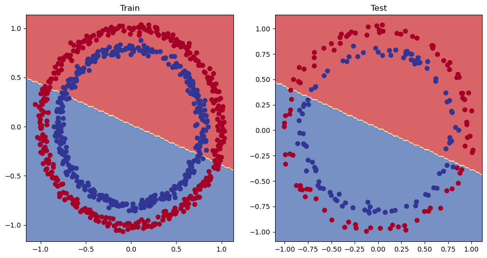
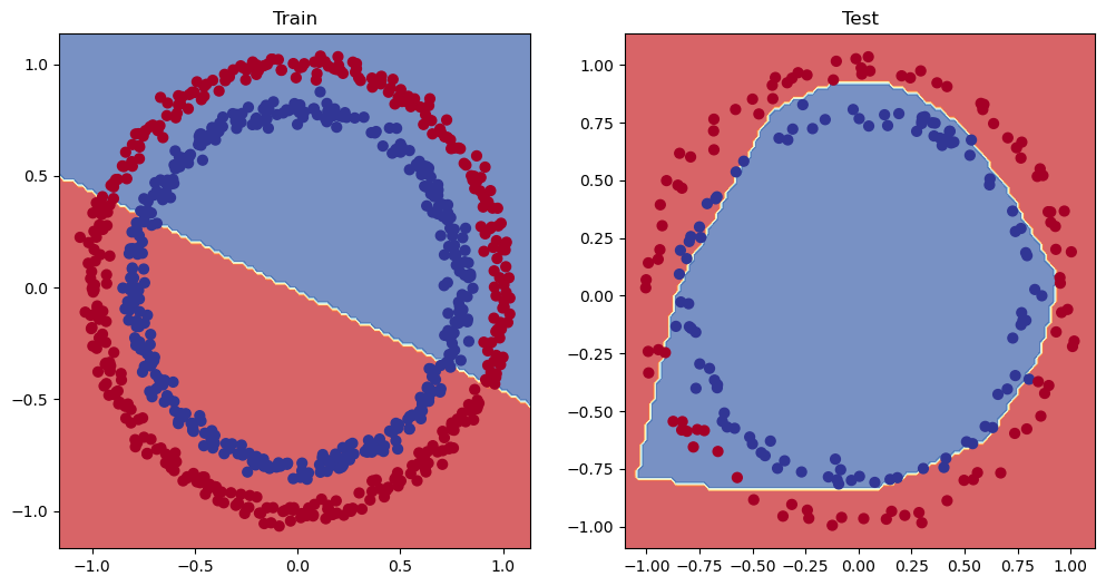
plt.figure(figsize=(12, 6))
plt.subplot(1, 2, 1)
plt.title("Train")
plot_decision_boundary(model_0, X_train, y_train)

plt.subplot(1, 2, 2)
plt.title("Test")
plot_decision_boundary(model_0, X_test, y_test)

PyTorch-26H-3-4

由于数据是圆形的，因此画一条直线最多只能将其从中间切开。

用机器学习术语来说，模型拟合不足underfitting，意味着它没有从数据中学习预测模式。

5. Improving a model (from a model perspective) 改进模型（从模型角度）

修复模型的欠拟合问题。

特别关注模型（而不是数据），我们可以通过几种方式来做到这一点。

模型改进技术	作用
添加更多层 Add more layers	每一层都可能增加模型的学习能力，因为每一层都能够学习数据中的某种新模式。更多层通常被称为使神经网络更深。
添加更多隐藏单元 Add more hidden units	与上述类似，每层隐藏单元越多，模型的学习能力就越强。更多隐藏单元通常被称为使神经网络更宽。
更长训练时间（更多循环） Fitting for longer (more epochs)	如果您的模型有更多机会查看数据，它可能会学到更多东西。
改变激活函数 Changing the activation functions	有些数据无法仅用直线来拟合（就像我们所看到的），使用非线性激活函数可以帮助解决这个问题（提示，提示）。
改变学习率 Change the learning rate	虽然与模型不太相关，但仍然相关，优化器的学习率决定了模型每一步应该改变多少参数，太多则模型过度修正，太少则学习不够。
改变损失函数 Change the loss function	同样，虽然模型特定性不强但仍然很重要，不同的问题需要不同的损失函数。例如，二元交叉熵损失函数不适用于多类分类问题。
使用迁移学习 Use transfer learning	从与您的问题领域类似的问题中获取预训练模型，并根据您自己的问题进行调整。

可以手动调整→超参数
机器学习为一半科学一半艺术，需要通过不断实验进行。

PyTorch-26H-3-5_1

让我们看看如果我们在模型中添加一个额外的层，适应更长的时间（epochs=1000 而不是 epochs=100），并将隐藏单元的数量从 5 增加到 10，会发生什么。

我们将遵循上述相同的步骤，但会更改一些超参数。

class CircleModelV1(nn.Module):
    def __init__(self):
        super().__init__()
        self.layer_1 = nn.Linear(in_features=2, out_features=10)
        self.layer_2 = nn.Linear(in_features=10, out_features=10) 
        self.layer_3 = nn.Linear(in_features=10, out_features=1)
        
    def forward(self, x): 
        
        
        
        
        
        
        return self.layer_3(self.layer_2(self.layer_1(x)))

model_1 = CircleModelV1().to(device)
model_1

CircleModelV1(
  (layer_1): Linear(in_features=2, out_features=10, bias=True)
  (layer_2): Linear(in_features=10, out_features=10, bias=True)
  (layer_3): Linear(in_features=10, out_features=1, bias=True)
)

现在我们有了一个模型，我们将使用与之前相同的设置重新创建一个损失函数和优化器实例。

1
2
3


loss_fn = nn.BCEWithLogitsLoss() 
optimizer = torch.optim.SGD(model_1.parameters(), lr=0.1)

这次我们将进行更长时间的训练（epochs=1000 vs epochs=100），看看它是否能改进我们的模型。

torch.manual_seed(42)
torch.cuda.manual_seed(42)

epochs = 1000 


X_train, y_train = X_train.to(device), y_train.to(device)
X_test, y_test = X_test.to(device), y_test.to(device)

for epoch in range(epochs):
    
    
    y_logits = model_1(X_train).squeeze()
    y_pred = torch.round(torch.sigmoid(y_logits)) 

    
    loss = loss_fn(y_logits, y_train)
    acc = accuracy_fn(y_true=y_train, 
                      y_pred=y_pred)

    
    optimizer.zero_grad()

    
    loss.backward()

    
    optimizer.step()

    
    model_1.eval()
    with torch.inference_mode():
        
        test_logits = model_1(X_test).squeeze() 
        test_pred = torch.round(torch.sigmoid(test_logits))
        
        test_loss = loss_fn(test_logits,
                            y_test)
        test_acc = accuracy_fn(y_true=y_test,
                               y_pred=test_pred)

    
    if epoch % 100 == 0:
        print(f"Epoch: {epoch} | Loss: {loss:.5f}, Accuracy: {acc:.2f}% | Test loss: {test_loss:.5f}, Test acc: {test_acc:.2f}%")

Epoch: 0 | Loss: 0.69396, Accuracy: 50.88% | Test loss: 0.69261, Test acc: 51.00%
Epoch: 100 | Loss: 0.69305, Accuracy: 50.38% | Test loss: 0.69379, Test acc: 48.00%
Epoch: 200 | Loss: 0.69299, Accuracy: 51.12% | Test loss: 0.69437, Test acc: 46.00%
Epoch: 300 | Loss: 0.69298, Accuracy: 51.62% | Test loss: 0.69458, Test acc: 45.00%
Epoch: 400 | Loss: 0.69298, Accuracy: 51.12% | Test loss: 0.69465, Test acc: 46.00%
Epoch: 500 | Loss: 0.69298, Accuracy: 51.00% | Test loss: 0.69467, Test acc: 46.00%
Epoch: 600 | Loss: 0.69298, Accuracy: 51.00% | Test loss: 0.69468, Test acc: 46.00%
Epoch: 700 | Loss: 0.69298, Accuracy: 51.00% | Test loss: 0.69468, Test acc: 46.00%
Epoch: 800 | Loss: 0.69298, Accuracy: 51.00% | Test loss: 0.69468, Test acc: 46.00%
Epoch: 900 | Loss: 0.69298, Accuracy: 51.00% | Test loss: 0.69468, Test acc: 46.00%

我们的模型训练的时间更长，并且增加了一层，但它看起来仍然没有学到比随机猜测更好的模式。


plt.figure(figsize=(12, 6))
plt.subplot(1, 2, 1)
plt.title("Train")
plot_decision_boundary(model_1, X_train, y_train)
plt.subplot(1, 2, 2)
plt.title("Test")
plot_decision_boundary(model_1, X_test, y_test)

PyTorch-26H-3-5

我们的模型仍然在红点和蓝点之间画一条直线。

如果我们的模型画的是直线，那么它能模拟线性数据吗？

5.1 Preparing data to see if our model can model a straight line 准备数据，看看我们的模型是否能建模直线

创建一些线性数据来看看我们的模型是否能够对其进行建模，而不仅仅是使用一个无法学习任何东西的模型。


weight = 0.7
bias = 0.3
start = 0
end = 1
step = 0.01


X_regression = torch.arange(start, end, step).unsqueeze(dim=1)
y_regression = weight * X_regression + bias 


print(len(X_regression))
X_regression[:5], y_regression[:5]

100
(tensor([[0.0000],
         [0.0100],
         [0.0200],
         [0.0300],
         [0.0400]]),
 tensor([[0.3000],
         [0.3070],
         [0.3140],
         [0.3210],
         [0.3280]]))

将数据分成训练集和测试集。


train_split = int(0.8 * len(X_regression)) 
X_train_regression, y_train_regression = X_regression[:train_split], y_regression[:train_split]
X_test_regression, y_test_regression = X_regression[train_split:], y_regression[train_split:]


print(len(X_train_regression), 
    len(y_train_regression), 
    len(X_test_regression), 
    len(y_test_regression))

1	80 80 20 20

漂亮，让我们看看数据是什么样子的。

为此，我们将使用我们在笔记本 01 中创建的 plot_predictions() 函数。

它包含在我们上面下载的 Learn PyTorch for Deep Learning 存储库中的 helper_functions.py 脚本中。

plot_predictions(train_data=X_train_regression,
    train_labels=y_train_regression,
    test_data=X_test_regression,
    test_labels=y_test_regression
)

PyTorch-26H-3-6

5.2 Adjusting `model_1` to fit a straight line 调整 `model_1` 以适合直线

重新创建model_1，但使用适合我们的回归数据的损失函数。


model_2 = nn.Sequential(
    nn.Linear(in_features=1, out_features=10),
    nn.Linear(in_features=10, out_features=10),
    nn.Linear(in_features=10, out_features=1)
).to(device)

model_2

Sequential(
  (0): Linear(in_features=1, out_features=10, bias=True)
  (1): Linear(in_features=10, out_features=10, bias=True)
  (2): Linear(in_features=10, out_features=1, bias=True)
)

将损失函数设置为nn.L1Loss()（与平均绝对误差相同），并将优化器设置为torch.optim.SGD()。

1
2
3


loss_fn = nn.L1Loss()
optimizer = torch.optim.SGD(model_2.parameters(), lr=0.1)

现在让我们使用常规训练循环步骤来训练模型，epochs=1000（就像model_1一样）。


torch.manual_seed(42)
torch.cuda.manual_seed(42)


epochs = 1000


X_train_regression, y_train_regression = X_train_regression.to(device), y_train_regression.to(device)
X_test_regression, y_test_regression = X_test_regression.to(device), y_test_regression.to(device)

for epoch in range(epochs):
    
    
    y_pred = model_2(X_train_regression)
    
    
    loss = loss_fn(y_pred, y_train_regression)

    
    optimizer.zero_grad()

    
    loss.backward()

    
    optimizer.step()

    
    model_2.eval()
    with torch.inference_mode():
      
      test_pred = model_2(X_test_regression)
      
      test_loss = loss_fn(test_pred, y_test_regression)

    
    if epoch % 100 == 0: 
        print(f"Epoch: {epoch} | Train loss: {loss:.5f}, Test loss: {test_loss:.5f}")

Epoch: 0 | Train loss: 0.75986, Test loss: 0.54143
Epoch: 100 | Train loss: 0.09309, Test loss: 0.02901
Epoch: 200 | Train loss: 0.07376, Test loss: 0.02850
Epoch: 300 | Train loss: 0.06745, Test loss: 0.00615
Epoch: 400 | Train loss: 0.06107, Test loss: 0.02004
Epoch: 500 | Train loss: 0.05698, Test loss: 0.01061
Epoch: 600 | Train loss: 0.04857, Test loss: 0.01326
Epoch: 700 | Train loss: 0.06109, Test loss: 0.02127
Epoch: 800 | Train loss: 0.05599, Test loss: 0.01426
Epoch: 900 | Train loss: 0.05571, Test loss: 0.00603

好的，与分类数据上的 model_1 不同，model_2 的损失似乎实际上在下降。

让我们绘制它的预测图，看看是否如此。

请记住，由于我们的模型和数据正在使用目标设备，并且该设备可能是 GPU，因此我们的绘图函数使用 matplotlib，而 matplotlib 无法处理 GPU 上的数据。

为了处理这个问题，当我们将所有数据传递给 plot_predictions() 时，我们将使用 .cpu() 将所有数据发送到 CPU。


model_2.eval()


with torch.inference_mode():
    y_preds = model_2(X_test_regression)



plot_predictions(train_data=X_train_regression.cpu(),
                 train_labels=y_train_regression.cpu(),
                 test_data=X_test_regression.cpu(),
                 test_labels=y_test_regression.cpu(),
                 predictions=y_preds.cpu());

PyTorch-26H-3-7

模型比在直线上随机猜测要好得多。这意味着我们的模型至少具有一定的学习能力。

构建深度学习模型时，一个有用的故障排除步骤是先从尽可能小的模型开始，看看模型是否有效，然后再将其扩大。
这可能意味着从一个简单的神经网络（层数不多，隐藏神经元也不多）和一个小的数据集（就像我们制作的数据集）开始，然后在这个小例子上进行过度拟合overfitting（使模型表现得太好了），然后再增加数据量或模型大小 / 设计以减少过度拟合。

6. The missing piece: non-linearity 缺失的部分：非线性

由于模型具有线性层，因此它可以绘制直线（线性）。

但是我们如何赋予它绘制非直线（非线性）线条的能力呢？

6.1 Recreating non-linear data (red and blue circles) 重新创建非线性数据（红色和蓝色圆圈）

重新创建数据以从头开始。我们将使用与之前相同的设置。


import matplotlib.pyplot as plt
from sklearn.datasets import make_circles

n_samples = 1000

X, y = make_circles(n_samples=1000,
    noise=0.03,
    random_state=42,
)

plt.scatter(X[:, 0], X[:, 1], c=y, cmap=plt.cm.RdBu);

PyTorch-26H-3-8

太棒了！现在让我们将其分成训练集和测试集，其中 80% 的数据用于训练，20% 的数据用于测试。


import torch
from sklearn.model_selection import train_test_split


X = torch.from_numpy(X).type(torch.float)
y = torch.from_numpy(y).type(torch.float)


X_train, X_test, y_train, y_test = train_test_split(X, 
                                                    y, 
                                                    test_size=0.2,
                                                    random_state=42
)

X_train[:5], y_train[:5]

(tensor([[ 0.6579, -0.4651],
         [ 0.6319, -0.7347],
         [-1.0086, -0.1240],
         [-0.9666, -0.2256],
         [-0.1666,  0.7994]]),
 tensor([1., 0., 0., 0., 1.]))

6.2 Building a model with non-linearity 建立非线性模型

可以用无限的直线（线性）和非直线（非线性）绘制什么样的图案？

到目前为止，我们的神经网络仅使用线性（直线）函数。

但我们处理的数据是非线性的（圆圈）。

当我们为模型引入使用非线性激活函数的能力时

PyTorch 有一堆现成的非线性激活函数，它们可以执行类似但不同的事情。

最常见且性能最好的一种是ReLU)（整流线性单元，torch.nn.ReLU()）。

将它放在神经网络中前向传递的隐藏层之间，看看会发生什么。


from torch import nn
class CircleModelV2(nn.Module):
    def __init__(self):
        super().__init__()
        self.layer_1 = nn.Linear(in_features=2, out_features=10)
        self.layer_2 = nn.Linear(in_features=10, out_features=10)
        self.layer_3 = nn.Linear(in_features=10, out_features=1)
        self.relu = nn.ReLU() 
        
        
        

    def forward(self, x):
      
       return self.layer_3(self.relu(self.layer_2(self.relu(self.layer_1(x)))))

model_3 = CircleModelV2().to(device)
print(model_3)

CircleModelV2(
  (layer_1): Linear(in_features=2, out_features=10, bias=True)
  (layer_2): Linear(in_features=10, out_features=10, bias=True)
  (layer_3): Linear(in_features=10, out_features=1, bias=True)
  (relu): ReLU()
)

与我们刚刚构建的分类神经网络（使用 ReLU 激活）类似的分类神经网络的视觉示例。尝试在 TensorFlow Playground 网站上创建一个您自己的神经网络。

问题：构建神经网络时，我应该把非线性激活函数放在哪里？
经验法则是将它们放在隐藏层之间，紧接着输出层，但是，没有一成不变的选择。随着您对神经网络和深度学习的了解越来越多，您会发现很多不同的组合方法。与此同时，最好不断实验、实验、再实验。

现在我们已经准备好了模型，让我们创建一个二元分类损失函数以及一个优化器。

1
2
3


loss_fn = nn.BCEWithLogitsLoss()
optimizer = torch.optim.SGD(model_3.parameters(), lr=0.1)

6.3 Training a model with non-linearity 训练非线性模型

训练、模型、损失函数、优化器已准备就绪，让我们创建一个训练和测试循环。


torch.manual_seed(42)
torch.cuda.manual_seed(42)
epochs = 1000


X_train, y_train = X_train.to(device), y_train.to(device)
X_test, y_test = X_test.to(device), y_test.to(device)

for epoch in range(epochs):
    model_3.train()
    
    
    y_logits = model_3(X_train).squeeze()
    y_pred = torch.round(torch.sigmoid(y_logits)) 
    
    
    loss = loss_fn(y_logits, y_train) 
    acc = accuracy_fn(y_true=y_train, 
                      y_pred=y_pred)
    
    
    optimizer.zero_grad()

    
    loss.backward()

    
    optimizer.step()

    
    model_3.eval()
    with torch.inference_mode():
      
      test_logits = model_3(X_test).squeeze()
      test_pred = torch.round(torch.sigmoid(test_logits)) 
      
      test_loss = loss_fn(test_logits, y_test)
      test_acc = accuracy_fn(y_true=y_test,
                             y_pred=test_pred)

    
    if epoch % 100 == 0:
        print(f"Epoch: {epoch} | Loss: {loss:.5f}, Accuracy: {acc:.2f}% | Test Loss: {test_loss:.5f}, Test Accuracy: {test_acc:.2f}%")

Epoch: 0 | Loss: 0.69295, Accuracy: 50.00% | Test Loss: 0.69319, Test Accuracy: 50.00%
Epoch: 100 | Loss: 0.69115, Accuracy: 52.88% | Test Loss: 0.69102, Test Accuracy: 52.50%
Epoch: 200 | Loss: 0.68977, Accuracy: 53.37% | Test Loss: 0.68940, Test Accuracy: 55.00%
Epoch: 300 | Loss: 0.68795, Accuracy: 53.00% | Test Loss: 0.68723, Test Accuracy: 56.00%
Epoch: 400 | Loss: 0.68517, Accuracy: 52.75% | Test Loss: 0.68411, Test Accuracy: 56.50%
Epoch: 500 | Loss: 0.68102, Accuracy: 52.75% | Test Loss: 0.67941, Test Accuracy: 56.50%
Epoch: 600 | Loss: 0.67515, Accuracy: 54.50% | Test Loss: 0.67285, Test Accuracy: 56.00%
Epoch: 700 | Loss: 0.66659, Accuracy: 58.38% | Test Loss: 0.66322, Test Accuracy: 59.00%
Epoch: 800 | Loss: 0.65160, Accuracy: 64.00% | Test Loss: 0.64757, Test Accuracy: 67.50%
Epoch: 900 | Loss: 0.62362, Accuracy: 74.00% | Test Loss: 0.62145, Test Accuracy: 79.00%

6.4 Evaluating a model trained with non-linear activation functions 评估用非线性激活函数训练的模型

还记得我们的圆形数据是非线性的吗？好吧，让我们看看现在模型的预测结果如何，该模型已经用非线性激活函数进行了训练。


model_3.eval()
with torch.inference_mode():
    y_preds = torch.round(torch.sigmoid(model_3(X_test))).squeeze()
y_preds[:10], y[:10]

1 2	(tensor([1., 0., 1., 0., 0., 1., 0., 0., 1., 0.], device='cuda:0'), tensor([1., 1., 1., 1., 0., 1., 1., 1., 1., 0.]))


plt.figure(figsize=(12, 6))
plt.subplot(1, 2, 1)
plt.title("Train")
plot_decision_boundary(model_1, X_train, y_train) 
plt.subplot(1, 2, 2)
plt.title("Test")
plot_decision_boundary(model_3, X_test, y_test)

PyTorch-26H-3-9

7. Replicating non-linear activation functions 复制非线性激活函数

您在自然中遇到的大部分数据都是非线性的（或线性和非线性的组合）。现在我们一直在处理二维图上的点。但想象一下，如果您有想要分类的植物图像，会有很多不同的植物形状。或者您想要总结的维基百科文本，有很多不同的单词组合方式（线性和非线性模式）。

但是非线性激活是什么样的？我们如何复制一些并看看它们的作用如何？

1
2
3


A = torch.arange(-10, 10, 1, dtype=torch.float32)
A

1 2	tensor([-10., -9., -8., -7., -6., -5., -4., -3., -2., -1., 0., 1., 2., 3., 4., 5., 6., 7., 8., 9.])

1 2	plt.plot(A);

PyTorch-26H-3-10

一条直线。

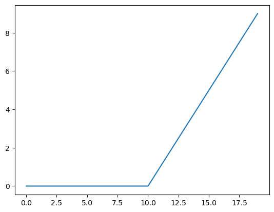
现在让我们看看 ReLU 激活函数如何影响它。

我们不会使用 PyTorch 的 ReLU (torch.nn.ReLU)，而是自己重新创建它。

ReLU 函数将所有负值变为 0，并保持正值不变。


def relu(x):
  return torch.maximum(torch.tensor(0), x) 


relu(A)

1 2	tensor([0., 0., 0., 0., 0., 0., 0., 0., 0., 0., 0., 1., 2., 3., 4., 5., 6., 7., 8., 9.])

看起来我们的 ReLU 函数起作用了，所有负值都是零。

1 2	plt.plot(relu(A));

PyTorch-26H-3-11

太棒了！这看起来和 ReLU 维基百科页面上的 ReLU 函数) 形状一模一样。

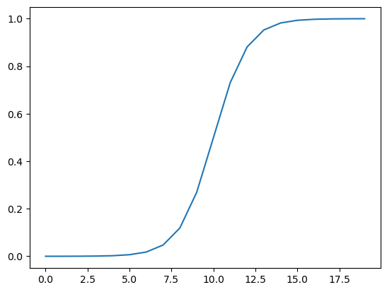
我们试试我们一直在使用的 sigmoid函数怎么样？

sigmoid 函数公式如下：

Or using $x$ as input:

其中 $S$ 代表 sigmoid 函数，$e$ 代表指数（torch.exp()），$i$ 代表张量中的特定元素。

让我们用 PyTorch 构建一个函数来复制 sigmoid 函数。


def sigmoid(x):
  return 1 / (1 + torch.exp(-x))


sigmoid(A)

tensor([4.5398e-05, 1.2339e-04, 3.3535e-04, 9.1105e-04, 2.4726e-03, 6.6929e-03,
        1.7986e-02, 4.7426e-02, 1.1920e-01, 2.6894e-01, 5.0000e-01, 7.3106e-01,
        8.8080e-01, 9.5257e-01, 9.8201e-01, 9.9331e-01, 9.9753e-01, 9.9909e-01,
        9.9966e-01, 9.9988e-01])

这些值看起来很像我们之前看到的预测概率，让我们看看它们的可视化效果。

1 2	plt.plot(sigmoid(A));

PyTorch-26H-3-12

看起来不错！我们已经从直线变成了曲线。

现在 PyTorch 中存在许多我们尚未尝试过的非线性激活函数。

但这两个是最常见的两个。

问题仍然存在，您可以使用无限数量的线性（直线）和非线性（非直线）线来绘制什么图案？

几乎任何东西都可以，对吗？

当我们结合线性和非线性函数时，这正是我们的模型所做的事情。

我们不是告诉模型要做什么，而是给它工具来找出如何最好地发现数据中的模式。

这些工具是线性和非线性函数。

8. Putting things together by building a multi-class PyTorch model 通过构建多类 PyTorch 模型将所有内容整合在一起

使用多类分类问题将它们放在一起。

二元分类问题是将某物归类为两个选项之一（例如，将一张照片归类为猫的照片或狗的照片）。而多类分类问题是从两个以上的选项列表中对某物进行分类（例如，将一张照片归类为猫、狗或鸡）。

8.1 Creating multi-class classification data 创建多类别分类数据

为了开始多类分类问题，让我们创建一些多类数据。

为此，我们可以利用 Scikit-Learn 的 make_blobs() 方法。

此方法将创建我们想要的任意数量的类（使用 centers 参数）。

具体来说，我们可以这样做：

1、使用 make_blobs() 创建一些多类数据。
2、将数据转换为张量（默认 make_blobs() 使用NumPy数组）。
3、使用 train_test_split() 将数据分为训练集和测试集。
4、使数据可视化。


import torch
import matplotlib.pyplot as plt
from sklearn.datasets import make_blobs
from sklearn.model_selection import train_test_split


NUM_CLASSES = 4
NUM_FEATURES = 2
RANDOM_SEED = 42


X_blob, y_blob = make_blobs(n_samples=1000,
    n_features=NUM_FEATURES, 
    centers=NUM_CLASSES, 
    cluster_std=1.5, 
    random_state=RANDOM_SEED
)


X_blob = torch.from_numpy(X_blob).type(torch.float)
y_blob = torch.from_numpy(y_blob).type(torch.LongTensor)
print(X_blob[:5], y_blob[:5])


X_blob_train, X_blob_test, y_blob_train, y_blob_test = train_test_split(X_blob,
    y_blob,
    test_size=0.2,
    random_state=RANDOM_SEED
)


plt.figure(figsize=(10, 7))
plt.scatter(X_blob[:, 0], X_blob[:, 1], c=y_blob, cmap=plt.cm.RdYlBu);

tensor([[-8.4134,  6.9352],
        [-5.7665, -6.4312],
        [-6.0421, -6.7661],
        [ 3.9508,  0.6984],
        [ 4.2505, -0.2815]]) tensor([3, 2, 2, 1, 1])

PyTorch-26H-3-13

准备好了一些多类数据。建立一个模型来分离彩色斑点。

问题：这个数据集需要非线性吗？或者你可以画出一系列直线来分离它吗？

8.2 Building a multi-class classification model in PyTorch 在 PyTorch 中构建多类分类模型

到目前为止，我们已经在 PyTorch 中创建了一些模型。

您或许还开始了解神经网络的灵活性。

PyTorch-26H-3-13_1

如何构建一个类似model_3但仍然能够处理多类数据的系统呢？

创建一个nn.Module包含三个超参数的子类：

input_features X 进入模型的特征数量。
output_features 我们想要的输出特征的理想数量（这将等同于NUM_CLASSES或等于多类分类问题中的类数）。
hidden_units 我们希望每个隐藏层使用的隐藏神经元的数量。

然后我们将使用上面的超参数创建模型类。

1
2
3


device = "cuda" if torch.cuda.is_available() else "cpu"
device

'cuda'

from torch import nn


class BlobModel(nn.Module):
    def __init__(self, input_features, output_features, hidden_units=8):
        """Initializes all required hyperparameters for a multi-class classification model.

        Args:
            input_features (int): Number of input features to the model.
            out_features (int): Number of output features of the model
              (how many classes there are).
            hidden_units (int): Number of hidden units between layers, default 8.
        """
        super().__init__()
        self.linear_layer_stack = nn.Sequential(
            nn.Linear(in_features=input_features, out_features=hidden_units),
            
            nn.Linear(in_features=hidden_units, out_features=hidden_units),
            
            nn.Linear(in_features=hidden_units, out_features=output_features), 
        )
    
    def forward(self, x):
        return self.linear_layer_stack(x)


model_4 = BlobModel(input_features=NUM_FEATURES, 
                    output_features=NUM_CLASSES, 
                    hidden_units=8).to(device)
model_4

BlobModel(
  (linear_layer_stack): Sequential(
    (0): Linear(in_features=2, out_features=8, bias=True)
    (1): Linear(in_features=8, out_features=8, bias=True)
    (2): Linear(in_features=8, out_features=4, bias=True)
  )
)

8.3 Creating a loss function and optimizer for a multi-class PyTorch model 为多类 PyTorch 模型创建损失函数和优化器

由于我们正在研究多类分类问题，我们将使用该nn.CrossEntropyLoss()方法作为我们的损失函数。

我们将坚持使用学习率为 0.1 的 SGD 来优化我们的model_4参数。


loss_fn = nn.CrossEntropyLoss()
optimizer = torch.optim.SGD(model_4.parameters(), 
                            lr=0.1)

8.4 Getting prediction probabilities for a multi-class PyTorch model 获取多类 PyTorch 模型的预测概率

准备好了损失函数和优化器，并且准备好训练我们的模型，但在此之前，让我们对我们的模型进行一次前向传递，看看它是否有效。

1 2	model_4(X_blob_train.to(device))[:5]

tensor([[-1.0821,  0.2580, -0.6953,  0.7268],
        [-0.4015,  2.0296,  2.3008,  1.7942],
        [ 1.3277, -0.3837,  0.2508, -1.6811],
        [ 0.7637,  0.1111,  0.5110, -0.8092],
        [-0.1890,  1.7277,  2.0414,  1.3623]], device='cuda:0',
       grad_fn=<SliceBackward0>)

为每个样本的每个特征都获得了一个值。检查一下形状以确认。

1 2	model_4(X_blob_train.to(device))[0].shape, NUM_CLASSES

1	(torch.Size([4]), 4)

模型正在为每个类别预测一个值。

你还记得我们模型的原始输出叫什么吗？

提示：它与“frog splits”押韵（在制作这些材料时没有伤害任何动物）。

如果你猜是 logits，那你就猜对了。

所以现在我们的模型正在输出 logits，但如果我们想弄清楚样本到底是哪个标签，该怎么办？

如何从 logits(raw output of model) -> prediction probabilities(use torch.softmax) -> prediction labels(take the argmax of the prediction probabilities)，就像我们处理二元分类问题一样？

这就是 softmax 激活函数发挥作用的地方。

softmax 函数计算每个预测类相对于所有其他可能类成为实际预测类的概率。



y_logits = model_4(X_blob_test.to(device))



y_pred_probs = torch.softmax(y_logits, dim=1) 
print(y_logits[:5])
print(y_pred_probs[:5])

tensor([[-1.2549, -0.8112, -1.4795, -0.5696],
        [ 1.7168, -1.2270,  1.7367,  2.1010],
        [ 2.2400,  0.7714,  2.6020,  1.0107],
        [-0.7993, -0.3723, -0.9138, -0.5388],
        [-0.4332, -1.6117, -0.6891,  0.6852]], device='cuda:0',
       grad_fn=<SliceBackward0>)
tensor([[0.1872, 0.2918, 0.1495, 0.3715],
        [0.2824, 0.0149, 0.2881, 0.4147],
        [0.3380, 0.0778, 0.4854, 0.0989],
        [0.2118, 0.3246, 0.1889, 0.2748],
        [0.1945, 0.0598, 0.1506, 0.5951]], device='cuda:0',
       grad_fn=<SliceBackward0>)

softmax 函数的输出可能看起来仍然是乱码（确实如此，因为我们的模型尚未经过训练，并且使用随机模式进行预测），但每个样本都有非常具体的区别。

将 logits 传递到 softmax 函数后，每个样本现在都加到 1（或非常接近）。

1
2
3



torch.sum(y_pred_probs[0])

1	tensor(1., device='cuda:0', grad_fn=<SumBackward0>)

这些预测概率本质上说明了模型认为目标 X 样本（输入）映射到每个类的程度。

由于 y_pred_probs 中每个类都有一个值，因此最高值的索引就是模型认为特定数据样本最属于的类。

我们可以使用 torch.argmax() 检查哪个索引具有最高值。



print(y_pred_probs[0])
print(torch.argmax(y_pred_probs[0]))

1
2
3

tensor([0.1872, 0.2918, 0.1495, 0.3715], device='cuda:0',
       grad_fn=<SelectBackward0>)
tensor(3, device='cuda:0')

您可以看到 torch.argmax() 的输出返回 3，因此对于索引 0 处的样本的特征 (X)，模型预测最可能的类值 (y) 是 3。

当然，现在这只是随机猜测，所以它有 25% 的正确率（因为有四个类）。但我们可以通过训练模型来提高这些机会。

模型的原始输出称为 logits。
对于多类分类问题，要将 logits 转换为预测概率，请使用 softmax 激活函数 (torch.softmax)。
具有最高预测概率的值的索引是模型认为在给定该样本的输入特征的情况下最有可能的类号（虽然这是一个预测，但并不意味着它是正确的）。

8.5 Creating a training and testing loop for a multi-class PyTorch model 为多类 PyTorch 模型创建训练和测试循环

好了，现在我们已经完成了所有准备步骤，让我们编写一个训练和测试循环来改进和评估我们的模型。

我们之前已经完成了很多这些步骤，所以其中很多都是练习。

唯一的区别是，我们将调整步骤，将模型输出（logits）转换为预测概率（使用softmax激活函数），然后转换为预测标签（通过取softmax激活函数输出的argmax）。

让我们训练模型epochs=100，并每10个epochs评估一次。


torch.manual_seed(42)
torch.cuda.manual_seed(42)


epochs = 100


X_blob_train, y_blob_train = X_blob_train.to(device), y_blob_train.to(device)
X_blob_test, y_blob_test = X_blob_test.to(device), y_blob_test.to(device)

for epoch in range(epochs):
    
    model_4.train()

    
    y_logits = model_4(X_blob_train) 
    y_pred = torch.softmax(y_logits, dim=1).argmax(dim=1) 
    
    
    loss = loss_fn(y_logits, y_blob_train) 
    acc = accuracy_fn(y_true=y_blob_train,
                      y_pred=y_pred)

    
    optimizer.zero_grad()

    
    loss.backward()

    
    optimizer.step()

    
    model_4.eval()
    with torch.inference_mode():
      
      test_logits = model_4(X_blob_test)
      test_pred = torch.softmax(test_logits, dim=1).argmax(dim=1)
      
      test_loss = loss_fn(test_logits, y_blob_test)
      test_acc = accuracy_fn(y_true=y_blob_test,
                             y_pred=test_pred)

    
    if epoch % 10 == 0:
        print(f"Epoch: {epoch} | Loss: {loss:.5f}, Acc: {acc:.2f}% | Test Loss: {test_loss:.5f}, Test Acc: {test_acc:.2f}%")

Epoch: 0 | Loss: 1.04324, Acc: 65.50% | Test Loss: 0.57861, Test Acc: 95.50%
Epoch: 10 | Loss: 0.14398, Acc: 99.12% | Test Loss: 0.13037, Test Acc: 99.00%
Epoch: 20 | Loss: 0.08062, Acc: 99.12% | Test Loss: 0.07216, Test Acc: 99.50%
Epoch: 30 | Loss: 0.05924, Acc: 99.12% | Test Loss: 0.05133, Test Acc: 99.50%
Epoch: 40 | Loss: 0.04892, Acc: 99.00% | Test Loss: 0.04098, Test Acc: 99.50%
Epoch: 50 | Loss: 0.04295, Acc: 99.00% | Test Loss: 0.03486, Test Acc: 99.50%
Epoch: 60 | Loss: 0.03910, Acc: 99.00% | Test Loss: 0.03083, Test Acc: 99.50%
Epoch: 70 | Loss: 0.03643, Acc: 99.00% | Test Loss: 0.02799, Test Acc: 99.50%Epoch: 0 | Loss: 1.04324, Acc: 65.50% | Test Loss: 0.57861, Test Acc: 95.50%
Epoch: 10 | Loss: 0.14398, Acc: 99.12% | Test Loss: 0.13037, Test Acc: 99.00%
Epoch: 20 | Loss: 0.08062, Acc: 99.12% | Test Loss: 0.07216, Test Acc: 99.50%
Epoch: 30 | Loss: 0.05924, Acc: 99.12% | Test Loss: 0.05133, Test Acc: 99.50%
Epoch: 40 | Loss: 0.04892, Acc: 99.00% | Test Loss: 0.04098, Test Acc: 99.50%
Epoch: 50 | Loss: 0.04295, Acc: 99.00% | Test Loss: 0.03486, Test Acc: 99.50%
Epoch: 60 | Loss: 0.03910, Acc: 99.00% | Test Loss: 0.03083, Test Acc: 99.50%
Epoch: 70 | Loss: 0.03643, Acc: 99.00% | Test Loss: 0.02799, Test Acc: 99.50%
Epoch: 80 | Loss: 0.03448, Acc: 99.00% | Test Loss: 0.02587, Test Acc: 99.50%
Epoch: 90 | Loss: 0.03300, Acc: 99.12% | Test Loss: 0.02423, Test Acc: 99.50%

8.6 Making and evaluating predictions with a PyTorch multi-class model 使用 PyTorch 多类模型进行预测并评估预测

看起来我们训练过的模型表现得相当不错。

但为了确保这一点，让我们做一些预测并将它们可视化。


model_4.eval()
with torch.inference_mode():
    y_logits = model_4(X_blob_test)


y_logits[:10]

tensor([[  4.3377,  10.3539, -14.8948,  -9.7642],
        [  5.0142, -12.0371,   3.3860,  10.6699],
        [ -5.5885, -13.3448,  20.9894,  12.7711],
        [  1.8400,   7.5599,  -8.6016,  -6.9942],
        [  8.0726,   3.2906, -14.5998,  -3.6186],
        [  5.5844, -14.9521,   5.0168,  13.2890],
        [ -5.9739, -10.1913,  18.8655,   9.9179],
        [  7.0755,  -0.7601,  -9.5531,   0.1736],
        [ -5.5918, -18.5990,  25.5309,  17.5799],
        [  7.3142,   0.7197, -11.2017,  -1.2011]], device='cuda:0')

看起来我们模型的预测仍然是 logit 形式。

但为了评估它们，它们必须与我们的标签 (y_blob_test) 具有相同的形式，后者是整数形式。

让我们将模型的预测 logit 转换为预测概率（使用 torch.softmax()），然后转换为预测标签（通过获取每个样本的 argmax()）。

可以跳过 torch.softmax() 函数，直接在 logits 上调用 torch.argmax()，从预测 logits -> predicted labels 直接进入。
例如，y_preds = torch.argmax(y_logits, dim=1)，这节省了一个计算步骤（没有 torch.softmax()），但导致没有可用的预测概率。



y_pred_probs = torch.softmax(y_logits, dim=1)



y_preds = y_pred_probs.argmax(dim=1)



print(f"Predictions: {y_preds[:10]}\nLabels: {y_blob_test[:10]}")
print(f"Test accuracy: {accuracy_fn(y_true=y_blob_test, y_pred=y_preds)}%")

1
2
3

Predictions: tensor([1, 3, 2, 1, 0, 3, 2, 0, 2, 0], device='cuda:0')
Labels: tensor([1, 3, 2, 1, 0, 3, 2, 0, 2, 0], device='cuda:0')
Test accuracy: 99.5%

模型预测现在与测试标签的形式相同。

使用 plot_decision_boundary() 将它们可视化，请记住，因为我们的数据在 GPU 上，所以我们必须将其移动到 CPU 以便与 matplotlib 一起使用（plot_decision_boundary() 会自动为我们执行此操作）。

plt.figure(figsize=(12, 6))
plt.subplot(1, 2, 1)
plt.title("Train")
plot_decision_boundary(model_4, X_blob_train, y_blob_train)
plt.subplot(1, 2, 2)
plt.title("Test")
plot_decision_boundary(model_4, X_blob_test, y_blob_test)

PyTorch-26H-3-14

9. More classification evaluation metrics 更多分类评估指标

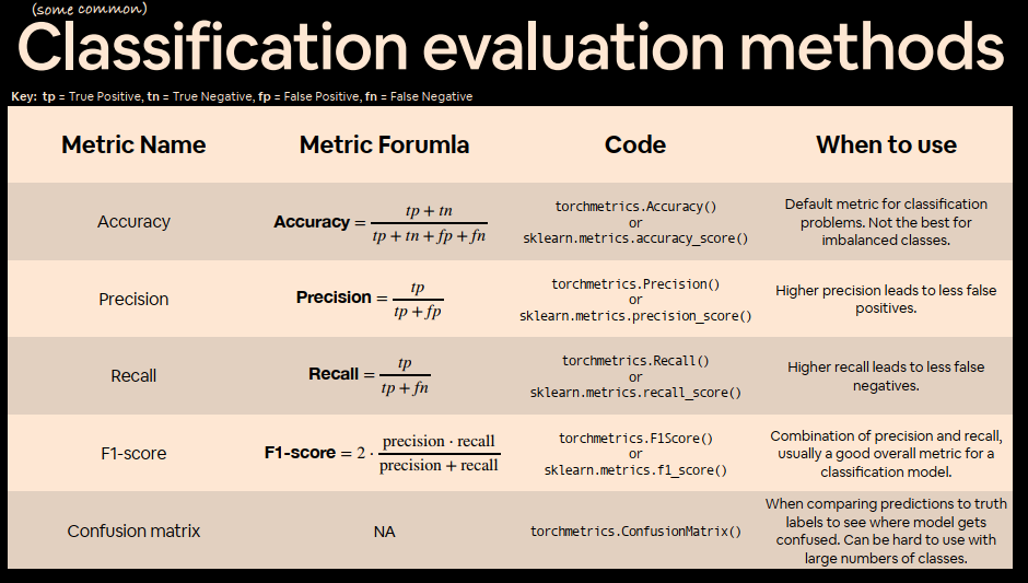
到目前为止，我们仅介绍了评估分类模型的几种方法（准确性、损失和可视化预测）。

这些是您会遇到的一些最常见的方法，并且是一个很好的起点。

可能希望使用更多指标来评估分类模型，例如：

Scikit-Learn（一个流行的、世界一流的机器学习库）对上述指标有许多实现，如果你正在寻找一个类似 PyTorch 的版本，请查看 TorchMetrics，尤其是 TorchMetrics 分类部分。

Precision 和 Recall 往往是相反的。

Beyond Accuracy: Precision and Recall

PyTorch-26H-3-15 PyTorch-26H-3-16

尝试一下 torchmetrics.Accuracy 指标。

try:
    from torchmetrics import Accuracy
except:
    !pip install torchmetrics==0.9.3 
    from torchmetrics import Accuracy


torchmetrics_accuracy = Accuracy(task='multiclass', num_classes=4).to(device)


torchmetrics_accuracy(y_preds, y_blob_test)

1	tensor(0.9950, device='cuda:0')

非线性激活函数

PyTorch-26H-3-17

Exercises

所有练习都集中于练习以上部分中的代码。

您应该能够通过参考每个部分或按照链接的资源来完成它们。

所有练习都应使用设备激动代码来完成。

资源：

练习模板笔记本02
02 的示例解决方案笔记本（在查看之前先尝试练习）

使用 Scikit-Learn 的函数创建二元分类数据集 make_moons()。
- 为了一致性，数据集应该有 1000 个样本和一个random_state=42。
- 将数据转换为 PyTorch 张量。将数据分为训练集和测试集，train_test_split其中 80% 用于训练，20% 用于测试。
通过子类化构建一个模型nn.Module，该模型包含非线性激活函数，并且能够拟合您在 1 中创建的数据。
- 请随意使用您想要的 PyTorch 层（线性和非线性）的任意组合。
设置二元分类兼容的损失函数和优化器，以便在训练模型时使用。
创建一个训练和测试循环，以使您在 2 中创建的模型适合您在 1 中创建的数据。
- 为了测量模型准确性，您可以创建自己的准确性函数或使用TorchMetrics中的准确性函数。
- 对模型进行足够长时间的训练，以达到 96% 以上的准确率。
- 训练循环应该每 10 个时期输出一次模型训练和测试集损失和准确率的进度。
使用训练好的模型进行预测，并使用plot_decision_boundary()此笔记本中创建的函数绘制它们。
在纯 PyTorch 中复制 Tanh（双曲正切）激活函数。
- 请随意参考ML 备忘单网站来获取该公式。
使用CS231n 中的螺旋数据创建功能创建多类数据集（代码见下文）。
- 构建一个能够拟合数据的模型（您可能需要线性和非线性层的组合）。
- 构建一个能够处理多类数据的损失函数和优化器（可选扩展：使用 Adam 优化器而不是 SGD，您可能必须尝试不同的学习率值才能使其发挥作用）。
- 对多类数据进行训练和测试循环，并在其上训练模型以达到 95% 以上的测试准确率（您可以在此处使用任何您喜欢的准确率测量函数）。
- 根据模型预测在螺旋数据集上绘制决策边界，该plot_decision_boundary()函数也适用于该数据集。


import numpy as np
N = 100 
D = 2 
K = 3 
X = np.zeros((N*K,D)) 
y = np.zeros(N*K, dtype='uint8') 
for j in range(K):
  ix = range(N*j,N*(j+1))
  r = np.linspace(0.0,1,N) 
  t = np.linspace(j*4,(j+1)*4,N) + np.random.randn(N)*0.2 
  X[ix] = np.c_[r*np.sin(t), r*np.cos(t)]
  y[ix] = j

plt.scatter(X[:, 0], X[:, 1], c=y, s=40, cmap=plt.cm.Spectral)
plt.show()

写下 3 个您认为机器分类可能有用的问题（可以是任何问题，您可以发挥创造力，例如，根据购买金额和购买地点特征将信用卡交易分类为欺诈或非欺诈）。
研究基于梯度的优化器（如 SGD 或 Adam）中的“动量”概念，它是什么意思？
花 10 分钟阅读Wikipedia 上关于不同激活函数的页面，其中有多少个你能与PyTorch 的激活函数相媲美？
研究何时准确度可能不是一个好的衡量标准（提示：阅读Will Koehrsen 的《超越准确度》来获取想法）。
观看：要了解我们的神经网络内部发生的情况以及它们如何学习，请观看麻省理工学院的深度学习简介视频。

推荐订阅源

HibisciDai

What is a classification problem? 什么是分类问题？

What we’re going to cover 我们将要讨论的内容

0. Architecture of a classification neural network 分类神经网络的架构

1. Make classification data and get it ready 分类数据制作及准备

1.1 Input and output shapes 输入和输出形状

1.2 Turn data into tensors and create train and test splits 将数据转换为张量并创建训练和测试分割

2. Building a model 建立模型

设置与设备无关的代码

通过子类化构建模型

Sequential 和 nn.model的区别

观察模型传递数据

定义损失函数和优化器

3. Train model

3.1 Going from raw model outputs to predicted labels (logits -> prediction probabilities -> prediction labels) 从原始模型输出到预测标签（logits -> 预测概率 -> 预测标签）

3.2 Building a training and testing loop 建立训练和测试循环

4. Make predictions and evaluate the model 做出预测并评估模型

5. Improving a model (from a model perspective) 改进模型（从模型角度）

5.1 Preparing data to see if our model can model a straight line 准备数据，看看我们的模型是否能建模直线

5.2 Adjusting `model_1` to fit a straight line 调整 `model_1` 以适合直线

6. The missing piece: non-linearity 缺失的部分：非线性

6.1 Recreating non-linear data (red and blue circles) 重新创建非线性数据（红色和蓝色圆圈）

6.2 Building a model with non-linearity 建立非线性模型

6.3 Training a model with non-linearity 训练非线性模型

6.4 Evaluating a model trained with non-linear activation functions 评估用非线性激活函数训练的模型

7. Replicating non-linear activation functions 复制非线性激活函数

8. Putting things together by building a multi-class PyTorch model 通过构建多类 PyTorch 模型将所有内容整合在一起

8.1 Creating multi-class classification data 创建多类别分类数据

8.2 Building a multi-class classification model in PyTorch 在 PyTorch 中构建多类分类模型

8.3 Creating a loss function and optimizer for a multi-class PyTorch model 为多类 PyTorch 模型创建损失函数和优化器

8.4 Getting prediction probabilities for a multi-class PyTorch model 获取多类 PyTorch 模型的预测概率

8.5 Creating a training and testing loop for a multi-class PyTorch model 为多类 PyTorch 模型创建训练和测试循环

8.6 Making and evaluating predictions with a PyTorch multi-class model 使用 PyTorch 多类模型进行预测并评估预测

9. More classification evaluation metrics 更多分类评估指标

非线性激活函数

Exercises

推荐订阅源

HibisciDai

What is a classification problem? 什么是分类问题？

What we’re going to cover 我们将要讨论的内容

0. Architecture of a classification neural network 分类神经网络的架构

1. Make classification data and get it ready 分类数据制作及准备

1.1 Input and output shapes 输入和输出形状

1.2 Turn data into tensors and create train and test splits 将数据转换为张量并创建训练和测试分割

2. Building a model 建立模型

设置与设备无关的代码

通过子类化构建模型

Sequential 和 nn.model的区别

观察模型传递数据

定义损失函数和优化器

3. Train model

3.1 Going from raw model outputs to predicted labels (logits -> prediction probabilities -> prediction labels) 从原始模型输出到预测标签（logits -> 预测概率 -> 预测标签）

3.2 Building a training and testing loop 建立训练和测试循环

4. Make predictions and evaluate the model 做出预测并评估模型

5. Improving a model (from a model perspective) 改进模型（从模型角度）

5.1 Preparing data to see if our model can model a straight line 准备数据，看看我们的模型是否能建模直线

5.2 Adjusting model_1 to fit a straight line 调整 model_1 以适合直线

6. The missing piece: non-linearity 缺失的部分：非线性

6.1 Recreating non-linear data (red and blue circles) 重新创建非线性数据（红色和蓝色圆圈）

6.2 Building a model with non-linearity 建立非线性模型

6.3 Training a model with non-linearity 训练非线性模型

6.4 Evaluating a model trained with non-linear activation functions 评估用非线性激活函数训练的模型

7. Replicating non-linear activation functions 复制非线性激活函数

8. Putting things together by building a multi-class PyTorch model 通过构建多类 PyTorch 模型将所有内容整合在一起

8.1 Creating multi-class classification data 创建多类别分类数据

8.2 Building a multi-class classification model in PyTorch 在 PyTorch 中构建多类分类模型

8.3 Creating a loss function and optimizer for a multi-class PyTorch model 为多类 PyTorch 模型创建损失函数和优化器

8.4 Getting prediction probabilities for a multi-class PyTorch model 获取多类 PyTorch 模型的预测概率

8.5 Creating a training and testing loop for a multi-class PyTorch model 为多类 PyTorch 模型创建训练和测试循环

8.6 Making and evaluating predictions with a PyTorch multi-class model 使用 PyTorch 多类模型进行预测并评估预测

9. More classification evaluation metrics 更多分类评估指标

非线性激活函数

Exercises

5.2 Adjusting `model_1` to fit a straight line 调整 `model_1` 以适合直线