On April 3, 2025, the US announced sweeping tariffs on Chinese imports. SPY dropped 4.8% that day. The next day, it dropped another 6%. Financial news ran the usual headline: markets rattled by geopolitical uncertainty.

Three months earlier, on August 5, 2024, the yen carry trade unwound. SPY dropped 3% in a single session. VIXY hit 65. Same headline: geopolitical uncertainty roils markets.

Both events got the same label. But if you actually pull the data and look at what moved, the two events have almost nothing in common. Gold surged in the tariff shock. In the yen unwind, it fell. Bonds rallied in the yen unwind. In the tariff shock, they sold off alongside equities.

Same label. Completely different markets.

To understand why, in this analysis we'll forensically pull apart three geopolitical events using Python and EODHD’s market data APIs. We'll track what moved, in what order, what the options market was pricing before spot prices moved, and what news sentiment was saying through all of it. The data tells a more specific story than the headlines did.

Table of Contents

• Prerequisites

• Setup: The Asset Basket and Data Source

• The Repricing Sequence Engine

• Options Data and IV Skew

• Composite Stress Score

• News Sentiment

• Event 1: Hamas Attack on Israel, Oct 7 2023

• Event 2: Yen Carry Unwind, Aug 5 2024

• Event 3: US-China Tariff Shock, Apr 2025

• Putting It All Together: The Heatmap

• Final Thoughts

Prerequisites

Before following along, you should be comfortable with basic Python and pandas. This article assumes you can read DataFrames, work with dictionaries, write simple functions, and understand basic return calculations.

You’ll also need:

• Python 3.9 or later

• An EODHD API key

• The following Python libraries: requests, pandas, numpy, and plotly

• Basic familiarity with ETFs like SPY, QQQ, GLD, TLT, and VIXY

• Some understanding of returns, volatility, implied volatility, options skew, correlation, and market sentiment

You don't need to be an options expert to follow the article. The options section uses one simple idea: if out-of-the-money puts become more expensive relative to at-the-money calls, the market is paying more for downside protection. We’ll use that as a rough fear signal, not as a full options pricing model.

The goal isn't to build a perfect geopolitical risk model. The goal is to show how different market data layers can help separate one type of shock from another.

Setup: The Asset Basket and Data Source

The asset basket is built around one question: which instruments reveal the most about how a shock is being interpreted by the market?

Broad equities (SPY, QQQ, IWM) show the scale of the selloff and which market cap segments are hit hardest. Sector ETFs (XLE, XLF, ITA, XLK) show where the economic consequence is being priced. Energy, financials, defense, and tech each respond differently depending on the nature of the shock. Safe havens (GLD, TLT, UUP) are the most diagnostic: how gold, bonds, and the dollar move relative to equities tells you what kind of fear the market is expressing. VIXY tracks implied volatility directly.

Together, these 11 assets produce a fingerprint for each event.

We've pulled data from EODHD’s historical EOD API. Each event gets a 30-day window on either side of the event date.

import requests
import pandas as pd
import numpy as np
import plotly.graph_objects as go
from plotly.subplots import make_subplots

api_key = 'your_eodhd_api_key'

events = {
    'oct7_attack': {
        'date': '2023-10-07',
        'label': 'Hamas Attack on Israel (Oct 2023)',
        'shock_type': 'confidence',
        'shock_label': 'Type 1 - Confidence Shock'
    },
    'yen_carry_unwind': {
        'date': '2024-08-05',
        'label': 'Yen Carry Unwind + Middle East Escalation (Aug 2024)',
        'shock_type': 'liquidity',
        'shock_label': 'Type 2 - Liquidity Shock'
    },
    'tariff_shock': {
        'date': '2025-04-03',
        'label': 'US-China Tariff Shock (Apr 2025)',
        'shock_type': 'structural',
        'shock_label': 'Type 3 - Structural Shock'
    }
}

assets = {
    'spy': 'SPY.US', 'qqq': 'QQQ.US', 'iwm': 'IWM.US',
    'xle': 'XLE.US', 'xlf': 'XLF.US', 'ita': 'ITA.US',
    'xlk': 'XLK.US', 'gld': 'GLD.US', 'tlt': 'TLT.US',
    'uup': 'UUP.US', 'vixy': 'VIXY.US'
}

def fetch_prices(ticker, start, end):
    url = f'https://eodhd.com/api/eod/{ticker}'
    params = {
        'from': start,
        'to': end,
        'api_token': api_key,
        'fmt': 'json'
    }
    r = requests.get(url, params=params)
    df = pd.DataFrame(r.json())
    df['date'] = pd.to_datetime(df['date'])
    df = df.set_index('date')[['adjusted_close']]
    df.columns = [ticker.split('.')[0].lower()]
    return df

def fetch_event_prices(event_date, lookback=30, lookahead=30):
    start = (pd.Timestamp(event_date) - pd.Timedelta(days=lookback)).strftime('%Y-%m-%d')
    end = (pd.Timestamp(event_date) + pd.Timedelta(days=lookahead)).strftime('%Y-%m-%d')
    frames = [fetch_prices(ticker, start, end) for ticker in assets.values()]
    return pd.concat(frames, axis=1)

event_prices = {name: fetch_event_prices(e['date']) for name, e in events.items()}

event_prices.keys()

This gives us three dataframes: one per event, each with 11 columns and roughly 60 rows covering the full window.

dict_keys(['oct7_attack', 'yen_carry_unwind', 'tariff_shock'])

All prices are adjusted close, which handles any splits or dividend distortions cleanly.

The Repricing Sequence Engine

Before looking at each event individually, we need a consistent way to measure what happened across all of them. The repricing sequence engine does three things: normalizes all asset prices to 100 at the event date so cross-asset comparison is clean, slices a tight window around the event, and ranks assets by the size of their T+1 move to identify what repriced fastest.

def normalize_to_event(df, event_date):
    event_date = pd.Timestamp(event_date)
    valid_dates = df.index[df.index >= event_date]
    anchor = valid_dates[0]
    normalized = df.div(df.loc[anchor]) * 100
    return normalized, anchor

def get_event_window(df, anchor, t_minus=5, t_plus=10):
    start_idx = df.index.get_loc(anchor) - t_minus
    end_idx = df.index.get_loc(anchor) + t_plus
    start_idx = max(start_idx, 0)
    return df.iloc[start_idx:end_idx + 1]

def repricing_leaderboard(window_df, anchor):
    anchor_idx = window_df.index.get_loc(anchor)
    post_event = window_df.iloc[anchor_idx:]
    cumulative_returns = (post_event / post_event.iloc[0] - 1) * 100
    t1_moves = cumulative_returns.iloc[1].abs().sort_values(ascending=False)
    return cumulative_returns, t1_moves

event_windows = {}
leaderboards = {}

for name, meta in events.items():
    df = event_prices[name]
    normalized, anchor = normalize_to_event(df, meta['date'])
    window = get_event_window(normalized, anchor)
    cumret, t1_rank = repricing_leaderboard(window, anchor)
    event_windows[name] = {'window': window, 'anchor': anchor, 'cumret': cumret}
    leaderboards[name] = t1_rank
    print(f"\n{meta['label']}")
    print(f'anchor date: {anchor.date()}')
    print('T+1 move ranking:')
    print(t1_rank.round(2))

Output:

Hamas Attack on Israel (Oct 2023)
anchor date: 2023-10-09
T+1 move ranking:
vixy    3.35
iwm     1.13
xlf     0.73
ita     0.72
qqq     0.55
spy     0.52
uup     0.24
gld     0.17
xlk     0.15
tlt     0.14
xle     0.12
Name: 2023-10-10 00:00:00, dtype: float64

Yen Carry Unwind + Middle East Escalation (Aug 2024)
anchor date: 2024-08-05
T+1 move ranking:
vixy    20.52
tlt      2.24
xlf      1.62
xlk      1.36
iwm      1.09
qqq      0.96
spy      0.92
gld      0.80
xle      0.61
ita      0.57
uup      0.32
Name: 2024-08-06 00:00:00, dtype: float64

US-China Tariff Shock (Apr 2025)
anchor date: 2025-04-03
T+1 move ranking:
vixy    19.97
xle      9.20
ita      8.44
xlf      7.32
xlk      6.59
qqq      6.21
spy      5.85
iwm      4.46
gld      2.34
uup      1.11
tlt      1.09
Name: 2025-04-04 00:00:00, dtype: float64

VIXY leads all three events at T+1, which makes sense. Volatility reprices faster than anything else. But look past VIXY and the rankings diverge completely.

In the Hamas attack, moves were small across the board. The largest non-VIXY move was IWM at 1.13%. In the yen carry unwind, TLT was the second biggest mover at 2.24%, bonds bid hard as a safe haven. In the tariff shock, every equity sector moved 4% to 9% while TLT moved just 1.09%, and gold came in at 2.34%.

Three events with three completely different repricing hierarchies. The T+1 leaderboard alone tells you something meaningful about what each market was actually pricing.

Note on the Oct 7 anchor: the attack happened on a Saturday. The first trading day was Monday, October 9, which is why the anchor is Oct 9 rather than Oct 7. This matters for the skew analysis later.

Options Data and IV Skew

Price data tells you what happened. Options data tells you what the market was willing to pay to protect against it.

The skew metric we compute here is straightforward: the difference between the average implied volatility of OTM puts (strikes at 90% to 97% of spot) and ATM calls (97% to 103% of spot). When this number rises, the market is paying a premium for downside protection relative to upside exposure. That is fear, quantified.

We pull SPY options data from EODHD's options EOD endpoint, paginating through the full dataset for each event window.

def fetch_options_all(ticker, start, end, exp_cap):
    url = 'https://eodhd.com/api/mp/unicornbay/options/eod'
    all_records = []
    offset = 0
    limit = 1000
    cols = None

    while True:
        params = {
            'filter[underlying_symbol]': ticker,
            'filter[tradetime_from]': start,
            'filter[tradetime_to]': end,
            'filter[exp_date_to]': exp_cap,
            'fields[options-eod]': 'type,exp_date,strike,volatility,tradetime',
            'page[limit]': limit,
            'page[offset]': offset,
            'api_token': api_key,
            'compact': 1
        }
        r = requests.get(url, params=params)
        payload = r.json()

        if 'meta' not in payload:
            print(f'unexpected response at offset {offset}: {list(payload.keys())}')
            break

        if cols is None:
            cols = [f.strip() for f in payload['meta']['fields']]

        batch = payload['data']
        all_records.extend(batch)

        total = payload['meta']['total']
        offset += limit
        if offset >= total or not batch:
            break

    df = pd.DataFrame(all_records, columns=cols)
    df['tradetime'] = pd.to_datetime(df['tradetime'])
    df['exp_date'] = pd.to_datetime(df['exp_date'])
    df['strike'] = pd.to_numeric(df['strike'], errors='coerce')
    df['volatility'] = pd.to_numeric(df['volatility'], errors='coerce')
    return df.dropna(subset=['volatility', 'strike']).query('volatility > 0')

def compute_skew(df, spot):
    df = df.copy()
    df['moneyness'] = df['strike'] / spot

    for expiry in sorted(df['exp_date'].unique()):
        sub = df[df['exp_date'] == expiry]
        otm_puts = sub[(sub['type'] == 'put') & (sub['moneyness'].between(0.90, 0.97))]
        atm_calls = sub[(sub['type'] == 'call') & (sub['moneyness'].between(0.97, 1.03))]
        if otm_puts.empty or atm_calls.empty:
            continue

        daily_skew = []
        for date, puts in otm_puts.groupby('tradetime'):
            calls = atm_calls[atm_calls['tradetime'] == date]
            if calls.empty:
                continue
            skew = puts['volatility'].mean() - calls['volatility'].mean()
            daily_skew.append({'date': date, 'skew': skew})

        if daily_skew:
            print(f'  using expiry: {expiry.date()}, {len(daily_skew)} days')
            return pd.DataFrame(daily_skew).set_index('date').sort_index()

    return pd.DataFrame()

spy_skew = {}

for name, meta in events.items():
    anchor = event_windows[name]['anchor']
    spot = event_prices[name].loc[anchor, 'spy']
    start = (anchor - pd.Timedelta(days=20)).strftime('%Y-%m-%d')
    end = (anchor + pd.Timedelta(days=5)).strftime('%Y-%m-%d')
    exp_cap = (pd.Timestamp(end) + pd.Timedelta(days=90)).strftime('%Y-%m-%d')
    raw = fetch_options_all('SPY', start, end, exp_cap)
    print(f'\n{meta["label"]} | total rows: {len(raw)}')
    skew_df = compute_skew(raw, spot)
    spy_skew[name] = skew_df
    print(skew_df)

Output:

Hamas Attack on Israel (Oct 2023) | total rows: 10435
  using expiry: 2023-11-17, 3 days
                skew
date                
2023-10-11  0.014164
2023-10-12  0.034279
2023-10-13  0.054055
unexpected response at offset 11000: ['errors']

Yen Carry Unwind + Middle East Escalation (Aug 2024) | total rows: 10660
  using expiry: 2024-10-18, 11 days
                skew
date                
2024-07-26  0.040748
2024-07-29  0.041219
2024-07-30  0.087402
2024-07-31  0.029824
2024-08-01  0.065074
2024-08-02  0.053369
2024-08-05  0.049848
2024-08-06  0.055957
2024-08-07  0.050664
2024-08-08  0.050283
2024-08-09  0.055462
unexpected response at offset 11000: ['errors']

US-China Tariff Shock (Apr 2025) | total rows: 10698
  using expiry: 2025-06-20, 18 days
                skew
date                
2025-03-14  0.042500
2025-03-17  0.029671
2025-03-18  0.027886
2025-03-19  0.029360
2025-03-20  0.026691
2025-03-21  0.008500
2025-03-24  0.013388
2025-03-25  0.022157
2025-03-26  0.012829
2025-03-27  0.009171
2025-03-28  0.026971
2025-03-31  0.036586
2025-04-01  0.022857
2025-04-02 -0.023000
2025-04-03  0.019729
2025-04-04  0.036729
2025-04-07  0.005257
2025-04-08  0.041543

A few observations worth noting before the event analysis. The Oct 7 dataset has only three data points, all post-event, due to limited options coverage for that period. The tariff shock dataset has the richest pre-event coverage, going back to March 14, nearly three weeks before the event. It also includes a negative skew reading on April 2, the day before the crash. We'll look at what each of these means in context when we get to the individual events.

Composite Stress Score

The skew signal alone has a weakness: it can spike for reasons unrelated to geopolitical stress. To make it more robust, we combine it with a second signal: the rolling 10-day correlation between SPY and GLD.

Under normal conditions, equities and gold are weakly correlated or negatively correlated. When stress builds, that relationship breaks down. Tracking the breakdown gives us a second, independent measure of market stress that doesn't depend on options pricing.

Both signals are z-scored before combining, so neither dominates due to scale differences. The correlation signal is inverted since falling correlation means rising stress. The composite is the average of the two.

def build_composite(event_name, skew_df, event_prices_df, anchor):
    prices = event_prices_df[['spy', 'gld']].copy()
    prices['corr'] = prices['spy'].rolling(10).corr(prices['gld'])

    def zscore(s):
        return (s - s.mean()) / s.std()

    skew_z = zscore(skew_df['skew'])
    corr_z = zscore(prices['corr'].dropna())

    corr_z = corr_z * -1

    combined = pd.concat([skew_z.rename('skew_z'), corr_z.rename('corr_z')], axis=1).dropna()
    combined['composite'] = combined.mean(axis=1)

    combined['stress_flag'] = combined['composite'] > 1.0

    return combined

composites = {}

for name, meta in events.items():
    anchor = event_windows[name]['anchor']
    skew_df = spy_skew[name]
    prices_df = event_prices[name]
    comp = build_composite(name, skew_df, prices_df, anchor)
    composites[name] = comp
    print(f"\n{meta['label']}")
    print(comp.round(3))

Output:

Hamas Attack on Israel (Oct 2023)
            skew_z  corr_z  composite  stress_flag
date                                              
2023-10-11  -1.003  -1.186     -1.094        False
2023-10-12   0.006  -1.316     -0.655        False
2023-10-13   0.997  -0.971      0.013        False

Yen Carry Unwind + Middle East Escalation (Aug 2024)
            skew_z  corr_z  composite  stress_flag
date                                              
2024-07-26  -0.808  -0.863     -0.835        False
2024-07-29  -0.776  -1.074     -0.925        False
2024-07-30   2.343  -0.559      0.892        False
2024-07-31  -1.546  -0.082     -0.814        False
2024-08-01   0.835   0.933      0.884        False
2024-08-02   0.044   2.117      1.081         True
2024-08-05  -0.194   1.977      0.892        False
2024-08-06   0.219   1.525      0.872        False
2024-08-07  -0.138   1.170      0.516        False
2024-08-08  -0.164   0.881      0.358        False
2024-08-09   0.186   0.371      0.278        False

US-China Tariff Shock (Apr 2025)
            skew_z  corr_z  composite  stress_flag
date                                              
2025-03-17   0.511   0.516      0.513        False
2025-03-18   0.398   0.493      0.445        False
2025-03-19   0.491   0.154      0.323        False
2025-03-20   0.322  -0.209      0.057        False
2025-03-21  -0.830  -1.023     -0.926        False
2025-03-24  -0.520  -0.999     -0.759        False
2025-03-25   0.035  -0.777     -0.371        False
2025-03-26  -0.556  -0.566     -0.561        False
2025-03-27  -0.787   0.096     -0.346        False
2025-03-28   0.340   1.093      0.716        False
2025-03-31   0.949   1.179      1.064         True
2025-04-01   0.080   1.309      0.694        False
2025-04-02  -2.824   1.190     -0.817        False
2025-04-03  -0.119   1.047      0.464        False
2025-04-04   0.958   0.119      0.539        False
2025-04-07  -1.035  -0.794     -0.915        False
2025-04-08   1.263  -1.274     -0.006        False

The stress flag threshold is set at 1.0. Two days get flagged across all three events: August 2, 2024, for the yen carry unwind, and March 31, 2025, for the tariff shock. Both are pre-event. The Oct 7 dataset is too sparse to produce a meaningful composite reading.

The Apr 2 row in the tariff shock is worth noting: skew_z of -2.824, the most negative skew reading in the entire dataset, pulling the composite negative despite the correlation signal remaining elevated. The options market was actively pricing more upside than downside on the day before the largest single-day SPY drop of 2025. That isn't a signal failure to brush past. We'll come back to it.

News Sentiment

The final data layer is news sentiment. EODHD's sentiment API generates a daily normalized score for each ticker derived from financial news coverage, ranging from -1 (strongly negative) to +1 (strongly positive). We pull SPY sentiment as a broad market proxy for the same windows used in the options analysis.

def fetch_sentiment(ticker, start, end):
    url = 'https://eodhd.com/api/sentiments'
    params = {
        's': ticker,
        'from': start,
        'to': end,
        'api_token': api_key,
        'fmt': 'json'
    }
    r = requests.get(url, params=params)
    data = r.json()
    key = ticker if ticker in data else ticker + '.US'
    if key not in data:
        return pd.DataFrame()
    df = pd.DataFrame(data[key])
    df['date'] = pd.to_datetime(df['date'])
    df = df.set_index('date')[['normalized']].rename(columns={'normalized': 'sentiment'})
    return df.sort_index()

event_sentiment = {}

for name, meta in events.items():
    anchor = event_windows[name]['anchor']
    start = (anchor - pd.Timedelta(days=20)).strftime('%Y-%m-%d')
    end = (anchor + pd.Timedelta(days=10)).strftime('%Y-%m-%d')
    sent_df = fetch_sentiment('SPY', start, end)
    event_sentiment[name] = sent_df
    print(f"\n{meta['label']}")
    print(sent_df)

Output:

Hamas Attack on Israel (Oct 2023)
            sentiment
date                 
2023-09-25      0.997
2023-09-26      0.986

Yen Carry Unwind + Middle East Escalation (Aug 2024)
            sentiment
date                 
2024-07-17     0.9340
2024-07-22     0.9460
2024-07-23     0.9550
2024-07-25     0.9925
2024-07-26     0.9860
2024-07-29     0.9850
2024-07-30     0.9630
2024-07-31     0.9950
2024-08-02     0.3350
2024-08-05     0.9780
2024-08-06     0.3603
2024-08-15     0.9980

US-China Tariff Shock (Apr 2025)
            sentiment
date                 
2025-03-14    -0.9890
2025-03-15     0.9930
2025-03-17    -0.7010
2025-03-18     0.9990
2025-03-20    -0.8900
2025-03-22     0.9950
2025-03-24     0.9600
2025-03-27     0.9830
2025-03-28     0.9917
2025-04-03     0.9365
2025-04-05     0.0130
2025-04-06     0.9990
2025-04-07     0.9870
2025-04-09     0.5460
2025-04-10     0.8079
2025-04-11     0.0929
2025-04-12    -0.9920
2025-04-13     0.0130

Two things stand out immediately. For the yen carry unwind, sentiment ranged between 0.934 and 0.995 from July 17 through July 31 while skew was already spiking on July 30 and the composite was building. Sentiment did not register the stress the options market was pricing. For the tariff shock, sentiment on April 3, the day SPY dropped 4.8%, was +0.9365. Strongly positive. The news cycle had no idea what was coming.

The October 7 sentiment data has only two data points from late September, both near +1.0. This predates the event by nearly two weeks and tells us nothing about market sentiment around the attack itself. Coverage is too thin for this event to contribute to the sentiment analysis.

Event 1: Hamas Attack on Israel, Oct 7 2023

The Hamas attack on October 7, 2023, was a major geopolitical shock. The market's response was not.

SPY closed up 0.64% on October 9 relative to the October 6 close. The anchor is Monday, October 9, because the attack happened on a Saturday. GLD and TLT both rallied. VIXY spiked to a T+1 move of 3.35%, modest compared to the 20% readings in the other two events. Within two weeks, most assets had drifted back toward pre-event levels.

The market's interpretation was specific: this was a regional conflict with limited direct economic transmission. Israel is not a major oil supplier, not a critical trade partner, and not deeply embedded in global supply chains in a way that would reprice earnings expectations. The uncertainty was real. The economic consequence was not.

That distinction shows up clearly in the safe haven behavior. GLD and TLT both up, UUP flat, equities essentially unchanged. When gold and bonds rally together while equities hold, the market is expressing classic flight-to-safety. Money moved into defensive assets as insurance against uncertainty, not as a response to any fundamental repricing.

The skew data for this event is limited to three post-event days: October 11, 12, and 13. Skew climbed steadily from 0.014 to 0.054 over those three days, consistent with the market pricing of ongoing uncertainty in the days following the attack.

But because the attack happened on a weekend and EODHD's options coverage for this period is thin, there is no pre-event skew data. We can't say whether the options market anticipated this event.

The composite is similarly sparse. Three data points, none flagged. There isn't enough data here to draw conclusions about early warning signals.

This is the weakest case study analytically. It stays in the analysis because the repricing fingerprint is informative and the contrast with the other two events is stark. The small moves, the clean flight-to-safety pattern, and the rapid recovery point to a specific kind of event: one where the market prices fear without pricing economic damage. That's a meaningful category even if the options data can't say more about it.

Event 2: Yen Carry Unwind, Aug 5 2024

The August 2024 event is the most analytically rich of the three. It's also the one where the data most clearly supports the idea that structured market signals were pricing stress before the crash arrived.

The repricing sequence tells an immediate story. VIXY exploded to a T+1 move of 20.52%. TLT was the second biggest mover at 2.24%, bid hard as a safe haven. Equities sold off across the board.

This is what a liquidity shock looks like. The Bank of Japan raised rates unexpectedly on July 31, triggering a massive unwind of yen carry trades.

The selling wasn't driven by a change in economic fundamentals. It was driven by positioning. Traders who had borrowed cheaply in yen to buy higher-yielding assets were forced to sell those assets simultaneously to cover their positions. The correlation between assets broke down because everything was being sold for the same mechanical reason.

Now look at what the skew data was doing before any of this:

On July 30, six days before the crash, skew spiked to 0.087. The highest reading in the entire pre-event window by a significant margin. It then compressed on July 31 before rising again on August 1 and 2. The crash hit on August 5.

That July 30 spike is the most important data point in this analysis. The BOJ rate decision that triggered the unwind came on July 31. The options market was pricing elevated downside risk the day before the trigger event, not after it. Someone, or more likely many someones, was paying up for SPY put protection before the news was public.

Now look at what sentiment was doing over the same period:

From July 17 through July 31, sentiment held between 0.934 and 0.995. Near maximum bullishness, every single day. On July 30, the same day skew spiked to 0.087, sentiment was 0.963. The news cycle was not concerned. The options market was.

Sentiment finally dropped to 0.335 on August 2, three days after the skew spike and three days before the crash. By that point, the options market had already been signaling stress for nearly a week.

The composite flagged August 2 as a stress day, driven primarily by the correlation breakdown signal. The SPY/GLD rolling correlation had been deteriorating since late July as gold started decoupling from equities. The composite didn't catch the July 30 skew spike cleanly because the skew signal compressed the day after, pulling the z-score back down. But the combination of a spiking skew on July 30 and a flagged composite on August 2 gave a two-stage warning before the August 5 crash.

The yen carry unwind is the clearest case in this analysis for the thesis that structured market signals carry information that news sentiment does not. The options market wasn't prescient. But it was pricing something that the headlines weren't.

Event 3: US-China Tariff Shock, Apr 2025

The April 2025 tariff shock is the most interesting event in this analysis, not because the signals worked, but because of where they failed.

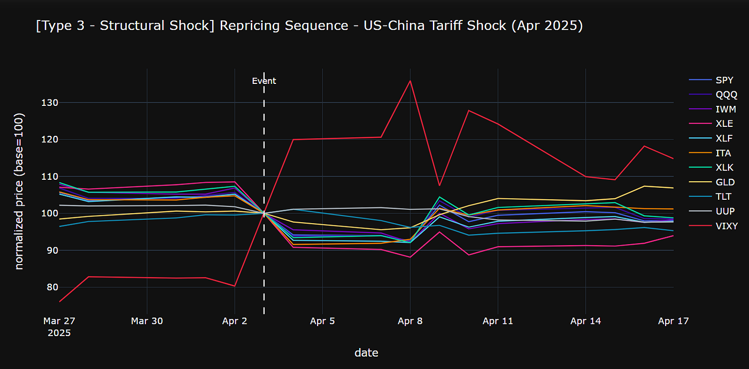
The numbers are severe. SPY dropped 5.85% at T+1 and continued falling through T+3. Every equity sector moved between 4% and 9%. XLE led at 9.20%, reflecting the direct exposure of energy and trade-dependent sectors to tariff policy. ITA followed at 8.44%. Tech dropped 6.59%.

These aren't volatility moves. They're repricing moves, the market adjusting its estimate of what these companies are actually worth under a structurally different trade regime.

The safe haven behavior is the most diagnostic part of this chart. GLD rose 2.34% at T+1 and kept climbing in the days that followed. TLT moved only 1.09% at T+1 and then sold off. Bonds and equities fell together. There was no flight to bonds. The only clean safe haven was gold.

This is what distinguishes a structural shock from the other two event types. In a confidence shock, both gold and bonds rally. In a liquidity shock, bonds rally hard. In a structural shock, bonds offer no protection because the shock itself calls into question the fiscal and monetary outlook. Gold becomes the only asset without a counterparty.

This is where the analysis gets genuinely uncomfortable.

On April 2, 2025, the day before the crash, skew was -0.023. Negative. ATM calls were more expensive than OTM puts. The options market wasn't pricing downside risk. It was pricing upside.

Skew had been elevated through mid-March, ranging from 0.025 to 0.042, then compressed steadily through late March. By the time the tariff announcement hit, the options market had actively de-risked its fear positioning.

There are two plausible explanations. The first is that the market had been pricing tariff risk as a negotiating tactic throughout March, then concluded by early April that a deal was likely. The negative skew on April 2 reflects collective confidence that the announced tariffs wouldn't materialize at full scale.

The second is that the options market simply didn't have the information. The tariff announcement on April 2 was more severe and more immediate than most participants expected.

Either way, the options market failed as an early warning signal here. This isn't a flaw in the methodology. It's a finding. Skew measures what market participants are willing to pay for protection. If participants have collectively decided a risk isn't worth pricing, skew won't warn you. That decision can be wrong.

The composite flagged March 31 as a stress day, three days before the crash. The signal came entirely from the correlation breakdown component, not the skew component. The SPY/GLD rolling correlation had been deteriorating through late March as gold climbed while equities softened. The composite picked up that decoupling even while skew was compressing.

On April 2, the composite dropped sharply to -0.817. The skew component had turned strongly negative, overwhelming the still-elevated correlation signal and flipping the composite well below zero. The composite effectively said no stress, just before the largest single-day SPY drop of 2025.

The tariff shock exposes a real limitation of any signal built on options pricing. When the market has collectively mispriced a risk, the signal will reflect that mispricing. The correlation breakdown component performed better here, but one signal out of two isn't a reliable composite.

Putting It All Together: The Heatmap

The individual event analyses show three different stories. The heatmap puts them side by side so the differences are visible in one place.

fig = make_subplots(rows=1, cols=3,
    subplot_titles=[e['label'] for e in events.values()],
    horizontal_spacing=0.08)

for i, (name, meta) in enumerate(events.items()):
    window = event_windows[name]['window']
    anchor = event_windows[name]['anchor']
    anchor_idx = window.index.get_loc(anchor)

    start_i = max(anchor_idx - 3, 0)
    end_i = min(anchor_idx + 8, len(window))
    slice_df = window.iloc[start_i:end_i].copy()
    slice_df.columns = [c.upper() for c in slice_df.columns]

    anchor_pos = anchor_idx - start_i
    anchor_vals = slice_df.iloc[anchor_pos]
    pct_df = ((slice_df - anchor_vals) / anchor_vals * 100).round(2)

    n_days = len(pct_df)
    t_labels = [f'T{d:+d}' for d in range(-anchor_pos, -anchor_pos + n_days)]

    fig.add_trace(go.Heatmap(
        z=pct_df.values.T,
        x=t_labels,
        y=list(pct_df.columns),
        colorscale='RdYlGn',
        zmid=0,
        zmin=-15,
        zmax=15,
        showscale=(i == 2),
        colorbar=dict(title='% return from T0')
    ), row=1, col=i+1)

fig.update_layout(
    title='Asset Return Heatmap - T-3 to T+7 across Events',
    template='plotly_dark',
    height=500
)

for annotation in fig['layout']['annotations']:
    annotation['font'] = dict(size=11)
    annotation['y'] = 1.02
    
fig.show()

Three panels, one per event, each showing percentage returns relative to the event date from T-3 to T+7. Green means the asset gained relative to T0. Red means it lost. The color scale is capped at plus or minus 15%, so the tariff shock’s extreme moves don't wash out the smaller Oct 7 moves.

The VIXY row tells different stories depending on the event. In the Hamas attack and tariff shock, it spikes green post-event as volatility surged above its T0 level. In the yen carry unwind, the row is deep red throughout, not because volatility didn't spike but because VIXY was already at its highest point on August 5, the anchor date, making everything relative to T0 look flat or negative.

Look at the GLD row. In the Hamas attack, it stays near neutral, a minimal safe haven response. In the yen carry unwind, it turns green post-event as forced selling cleared and gold recovered. In the tariff shock, it turns deeply green and stays there, the strongest and most sustained move of any asset across the three events.

The TLT row shows the starkest contrast. Near neutral in the Hamas attack, clearly green in the yen carry unwind as bonds rallied hard, and near neutral to slightly negative in the tariff shock. Bonds were a reliable safe haven in one event and offered almost nothing in the other two.

The equity rows tell the scale story. In the Hamas attack, the colors are pale, with small moves in both directions. In the yen carry unwind, they're moderately red before recovering to green. In the tariff shock, they are deep red across every sector from T0 through T+3, the kind of uniform selloff that happens when the market is repricing fundamentals, not just pricing fear.

This is what the taxonomy looks like in data form. Three events, three fingerprints, and three different markets responding to three different things that all got filed under the same label.

Final Thoughts

The three events in this analysis all got the same label. But the data gave them three different ones.

A confidence shock prices fear without pricing economic damage. Gold and bonds rally, equities hold, recovery is faster than it feels.

A liquidity shock is mechanical: everything sells off because positioning unwinds, not because fundamentals changed.

A structural shock reprices what companies are actually worth under a different economic regime. Bonds offer no protection. Gold is the only clean hedge. Recovery timeline is unknown.

The IV skew and correlation composite built here using EODHD’s historical and options data worked cleanly for one event, partially for another, and failed for the third. That's not a reason to dismiss the signals. It's a reason to understand what they measure. Skew reflects what participants are paying for downside protection. When the market has collectively decided a risk isn't worth pricing, skew goes quiet. That silence isn't safety.

The most useful output of this framework isn't a signal. It's a question: what kind of shock is this? The answer changes everything that follows.