By Evan Miller

July 14, 2022

So you’re running experiments and you heard about this CUPED thing, a thingamaquation that makes data scientists’ hearts beat quicker and FAANG experiments run faster, somehow, using math. You download the Controlled Experiments Using Pre-Existing Data paper and think to yourself, this doesn’t make any sense; or at least that was my experience, until I realized the CUPED authors had simply reinvented partial linear regressions, perhaps without knowing it.

Today we’re going to talk about the Frisch-Waugh-Lovell Theorem, a neat little nugget from 1933, and what it has to do with reducing sample sizes in experiments today, and why you should probably include a vector of treatments in your CUPED regressions to achieve Even More Variance Reduction than what the folks at FAANG are doing, at least in their published research.

Before we dive into the fancy stuff, let’s talk about a bit about variance reduction, and what it has to do with turning gray into green on your company’s experiment dashboard.

Sample Sizes and \(\sigma^2\)

It all starts with this equation:

\[ N=16\sigma^2/\delta^2 \]

The sordid origin of that formula is a story for another TikTok, but \(\sigma^2\) is the variance in the measured outcome, \(\delta\) is your good friend the Minimum Detectable Effect, and \(N\) is the number of lab rats you’ll need to drop into each cardboard box to achieve a given level of statistical power for your experiment.

Want to make \(N\) smaller and RUN EXPERIMENTS FASTER? The \(16\) out front isn’t going anywhere¹, so you’re left with two choices: squeeze down the numerator, or inflate the denominator. Increasing \(\delta\) (the MDE) reduces your ability to detect small treatment effects, maybe not what the website team wants to hear; decreasing \(\sigma^2\) is a byword for Variance Reduction, which is how data scientists cut down sample sizes and secure pay raises. \(\sigma^2\) is a measurement of the amount of noise in the data, and removing that noise leaves you with a cleaner signal about the effectiveness of your treatments. Sounds like a good plan, eh?

If this were a normal CUPED blog post, at this point I’d start talking about how we can use linear regression to change the outcome variable to something slightly less jiggly – and voila, variance reduction. But a normal post this is not, so we’re going to take a circuitous route to Rome, and cross paths with a Norwegian silversmith along the way.

Let’s backtrack and think a little bit harder about the \(\sigma^2\) term in the sample size equation. It’s “variance of the outcome” – but how is the variance measured, exactly?

To get specific, suppose you just finished running an experiment, and want to use the data from that experiment for your next sample size calculation. You look at \(\sigma^2\) from your completed experiment in three different ways:

	\(N\)	\(\sigma^2\)
Control	10,000	4.0
Treatment	10,000	4.2
Combined	20,000	16.5

Well hmm… which of these three \(\sigma^2\)’s belongs the magic sample size equation? And how is it that the combined \(\sigma^2\) is greater than the \(\sigma^2\) of the treatment and control?

Let’s start with the second question. It helps to look at the data from this fake experiment:

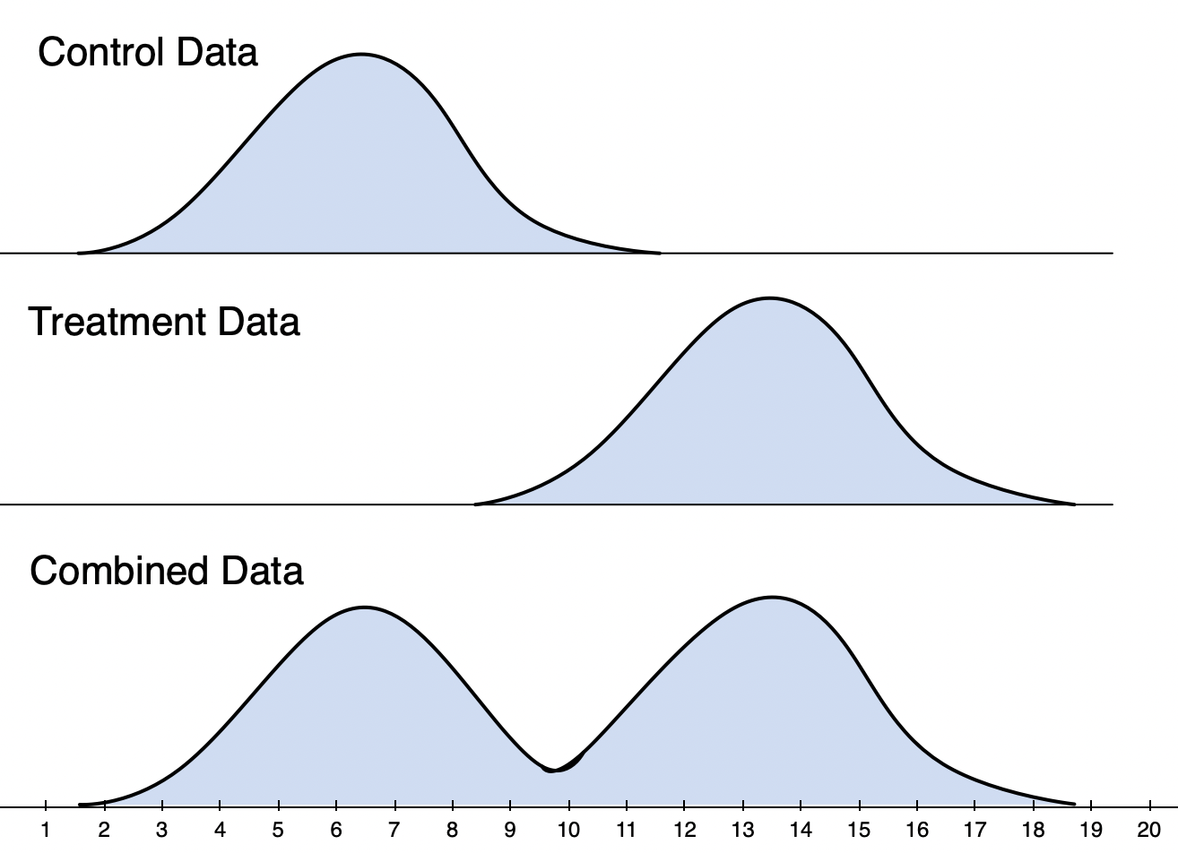
The picture should make it clear: with a strong treatment effect present, combining the two groups “creates” more variance than exists in either treatment or control.

There’s a specific mathematical relationship between the size of the treatment effect \(T\) and the three variance figures. It’s known as the law of total variance:

\[ \sigma^2_{combined}=\frac{1}{2}(\sigma^2_{control}+\sigma^2_{treatment})+\frac{1}{4}T^2 \]

This law lets us decompose the combined variance into two pieces: the variance within the two groups, and the variance between the groups. (Write down the variance formula to figure out why the between-group variance is equal to \(\frac{1}{4}T^2\).) You can see from the formula how the existence of a treatment effect, whether positive or negative, will always add variance to the combined sample.

The ANOVA test, which forms the basis of the mighty t-test and most A/B tests, is an implementation of the law of total variance. It “pulls out” the variance added by the treatment effect, and analyzes \(T\) using only the variance that remains within treatment and within control. In other words, the anticipated treatment effect of the next experiment should enter into the sample-size equation only through \(\delta\), and not through \(\sigma^2\).

(The which-sigma question that I posed above is a bit of a trick: the estimate of the next-experiment variance depends on whether the treatment or control was actually implemented, or whether the previous experiment is still ongoing. Later in this post, we’ll use the insight that experiments introduce variance to invent a new variance-reduction technique.)

Now let’s talk about reducing within-group variance by adding some covariates into ANOVA. I’m speaking, of course, of “the automobile of econometrics”: multiple regression, or ordinary least squares (OLS).

CUPED and Covariates

Thus far, we have modeled the experiment outcome \(Y\) as a treatment effect \(T\) (between-group variance) and some noise (within-group variance). To add some structure to the problem, let’s assume that the noise is normally distributed, and that the within-group variance is the same in both treatment and control:

\[ Y_{control}\sim N(\mu, \sigma^2) \] \[ Y_{treatment}\sim N(\mu+T, \sigma^2) \]

Instead of the usual t-test, we can then think about estimating \(T\) using a linear regression that includes observations from both treatment and control, which we can distinguish with an indicator variable \(1_{treated}\) (set to zero for control and one for treatment):

\[ Y=\mu+T\times 1_{treated}+\epsilon \] \[ \epsilon\sim N(0, \sigma^2) \]

Estimating the above equation with least-squares, we’ll get a t-statistic on \(T\) that is identical to a simple two-group, equal-variance t-test that you learned about in Stat 101. If you recall your OLS fundamentals, the variance of regression residuals are a consistent estimator of the conditional outcome variance. So to plan our next experiment, we can just compute the variance of the regression residuals, call it \(\hat{\sigma}^2\), then plug that into the numerator of the sample size formula.

What’s the point of all these regression gymnastics? Simple: if we can somehow figure out a way to reduce \(\hat{\sigma}^2\) in the regression, then the number of samples \(N\) required to achieve statistical significance is correspondingly smaller. This is the essence of variance reduction.

Suppose now that we have access to an additional \(Z\) that is correlated with \(\epsilon\), but not with the treatment assignment. Then we can pile those extra dishes on top of the kitchen-sink linear equation:

\[ Y=\mu+Z\beta+T\times 1_{treated} + \epsilon^* \]

Fitting \(\mu\), \(\beta\), and \(T\) with least squares, if \(\beta\) comes out non-zero, then the estimated variance of \(\epsilon^*\) in will come out smaller than the estimated variance of vanilla \(\epsilon\) – and voila, smaller \(N\) in the sample-size formula.

If you don’t trust the sample-size heuristic, you can also look at how \(\sigma^2\) affects the standard error of the \(T\) estimate, which will sit in the bottom-right corner of the well-known OLS variance-covariance matrix:

\[ Var\left(\begin{bmatrix}\mu \\\beta\\T\end{bmatrix}\right)=\sigma^2(\begin{bmatrix}1 \space Z \space 1_{treated}\end{bmatrix}'\space \begin{bmatrix}1 \space Z \space 1_{treated}\end{bmatrix})^{-1} \]

You can see that the entire right-hand side of the equation scales with \(\sigma^2\). Smaller \(\sigma^2\) yields tighter bounds on the whole vector of estimates; tighter bounds on \(T\) specifically means we have a cleaner signal on the treatment effect.²

What is this magic \(Z\) factor that is correlated with \(\epsilon\), but not with the treatment assignment? In the context of online experiments, some good candidates are previous values of \(Y\), or any user attributes that might influence \(Y\). (Country might be an easy one, if you’re running a globally-accessible website.)

If this sounds like CUPED, well, we’re almost there. The CUPED paper proposes running two separate analyses. In the first step, it predicts the outcome from a number of covariates, like this:

\[ Y=X\beta+\epsilon \]

In the second step, it takes the residuals from that regression \(\hat{u}=(Y - X\hat{\beta})\) and runs a t-test on treatment versus control. A t-test is equivalent to a simple linear regression, so we can write the second step as a univariate regression:

\[ \hat{u}=T\times1_{treated}+e \]

Now here’s a result that will come as a shock to anyone who hasn’t taken first-year econometrics: the t-statistic on the CUPED t-test will have the exact same asymptotic distribution as the t-statistic on the treatment variable in the combined least-squares regression.

Let that sink in for a moment, or several years.

Frisch-Waugh-Lovell and VaReSE

Ragnar Frisch and Frederick Waugh published the relevant result in the fourth issue of Econometrica back in 1933. Incidentally, Frisch, an economist from Norway who also happened to train as a silversmith, coined the term econometrics and later won the first Nobel Prize in Economics. So maybe it’s worth paying attention to. Michael Lovell extended Frisch and Waugh’s result in the 1960s, plastering his name on the now-famous Frisch-Waugh-Lovell theorem, and more recently published a simple proof of it here.

What do we do with the Frisch-Waugh-Lovell theorem? Well, a couple of things. First, it’s not necessary to perform CUPED in two steps. A statistically identical hypothesis test can be performed just by including the treatment indicator in the first regression and testing it for significance.³ I’ll reproduce the combined specification just so you have it handy:

\[ Y=\mu + Z\beta + T\times1_{treated}+\epsilon \]

Unless you’re dealing with massive matrices or something, there is no reason to split the analysis in two.

The second implication is where things get a little more interesting. By reformulating CUPED as a regression with covariates and a treatment effect, we can push the variance reduction further than the CUPED authors advertised as being possible.

Remember the side-tour above about treatment effects (between-group variance) contributing to total variance? Any experiment, by definition, is a potential source of variance in the outcome. (That’s the whole point of running experiments!) Using this linear-regression framework, we can modify the combined equation to include not just a single assignment variable, but the full vector of treatment assignments from all of the \(K\) experiments that are running simultaneously:

\[ Y=\mu+Z\beta+T_1+T_2+\ldots+T_K+\epsilon \]

(Indicator variables omitted for clarity.) As long as the assignments are uncorrelated, that is, properly randomized, the estimates of the treatment effects will remain unbiased, but the standard errors will be smaller than they were with separate regressions.

A linear regression with a treatment vector and CUPED covariates neatly decomposes the outcome variance into three parts: the variance introduced by the experiments, the variance introduced by the covariates, and the residual or unexplained variance. Including effective (\(T\ne0\)) experiments into the treatment vector necessarily reduces the residual variance, and therefore produces larger t-statistics on the entire vector of treatment effects. Cue the singing of the statistics angels, and a fresh infusion of color into the experiment dashboard.

The usual advice with running concurrent experiments is “don’t worry, the other treatment effects will balance each other out.” This is true insofar with regard to the estimates, but it’s not true with regard to the variance, which is additive. So if you’re running experiments concurrently, but analyzing them in isolation, you’re missing an opportunity to pull out the outcome variance that each experiment is introducing into all the contemporaneous experiments.

If you need a nifty Italianate acronym for the above method, may I suggest VaReSE: Variance Reduction in Simultaneous Experiments.

What’s the potential reduction in variance and therefore future sample sizes with VaReSE? In light of the law of total variance, the percent reduction will equal the sum of all the between-group variances for a given round of experiments divided by the residual variance from CUPED. To make an equation out of the preceding sentence:

\[ \Delta_{VaReSE} = \frac{\sum_k \frac{1}{4}T_k^2}{\sigma^2_{CUPED}} \]

Depending on the maturity of the experimentation operation, a sample-size reduction of a few percent seems achievable. Notice that this technique benefits from including experiments with negative as well as positive effects; as long as experiments are a source of variance, multiple regression can account for that additional noise.

As a final implementation note, you’ll probably want to flip on White standard errors in order to account for treatments whose within-group variance differs from the control, the same as Welch’s t-test does.

Conclusion

If multiple regression seems like sorcery, the Frisch-Waugh-Lovell theorem is a key cat-tail in the cauldron. It’s worth studying on its own, as it helps develop intuition about residuals and variance-accounting in nested regression models. If the authors of the original CUPED paper had written about this connection back in 2013, I feel certain their ideas would have come across more clearly. For an accessible treatment of regression anatomy, check out the book Mostly Harmless Econometrics. For something more heavy-duty, “all the math’s in Goldberger,” as my grizzled econometrics professor often repeated.

In the context of online experiments, Student’s traditional t-test is, quite literally, a waste of everyone’s time. Perhaps it’s finally time to sing Auld Lang Syne to it, and embrace multiple linear regression for its smaller standard errors and reduced sample sizes via CUPED – and its good-looking new neighbor, VaReSE. Multiple regression also gives you an elegant way to test complex hypotheses along the lines of, “Are the sum of these treatment effects greater than X?” Even with millions of users in a data set, these analyses run on modern hardware in under a second. So if you’re serious about learning from experiments, and doing it quickly, there’s really no excuse not to be running least squares.⁴

Postscript

If you enjoyed this post, please send a LinkedIn message to my boss and tell him that you absolutely love my marketing slogan for Eppo:

Frisch-Waugh-Lovell, Frisch-Waugh-Lovell, Frisch-Waugh-Lovell: Say it three times fast to run experiments three times faster.

Or maybe I’ll stick to statistics…

---

Notes

1. NIST’s Engineering Statistics Handbook has a discussion, but the heuristic constant comes from \((z_{1-\alpha/2}+z_{1-\beta})^2 \approx 8\) at standard 5% significance and 80% power.
2. The real reason that this argument works is that \(Z\) is uncorrelated with \(1_{treated}\), so the bottom-right corner of the inverted matrix will be unaffected in the limit after \(Z\) is inserted.
3. I’m glossing over some details, but in fact the FWL theorem shows how to obtain the exact, down-to-eight-decimals coefficient in the second regression. First regress the treatment indicator on the other covariates; then use the residuals from that regression in the second regression corresponding to our t-test. If the randomization is correct, then the true coefficients on the treatment regression will be zero. In practice, the estimates won’t be zero exactly – and the obtained “treatment residuals” will be slightly perturbed from zero and one, and so the final measured treatment effects from the regression and from the CUPED t-test will differ slightly. But both measurements will be consistent estimators of the same thing. For purposes of hypothesis testing, they’re interchangeable.
4. Unless, that is, you’ve implemented your entire experiment platform in JavaScript.

---

You’re reading evanmiller.org, a random collection of math, tech, and musings. If you liked this you might also enjoy:

• How Not To Run an A/B Test
• The Low Base Rate Problem
• Simple Sequential A/B Testing

---

Get new articles as they’re published, via LinkedIn, Twitter, or RSS.

---

Want to look for statistical patterns in your MySQL, PostgreSQL, or SQLite database? My desktop statistics software Wizard can help you analyze more data in less time and communicate discoveries visually without spending days struggling with pointless command syntax. Check it out!

Wizard
Statistics the Mac way

---

Back to Evan Miller’s home page – Subscribe to RSS – LinkedIn – Twitter

---