


A lot has happened in transformer quantization over the past few years, from barely being able to quantize a 7B model in INT8 without destroying accuracy, to routinely fitting a 70B model in 4-bits on a single GPU. But existing guides on the topic are fragmented: either focused on a specific technique or on how to use a library. I’ve been working on integer quantization for fixed-point hardware for a while now and my goal with this series is to bridge that gap: building the core ideas carefully and tracing how the field has evolved, each technique motivated by the problems of what came before. This first post covers the foundations: what quantization is, why it’s hard, and the math behind it.
Quantization is the process of representing high-precision values using fewer bits. In practice, this means storing weights and (optionally) activations in lower precision (e.g., int8 instead of fp16), introducing a small approximation error.
The most immediate and easy-to-realize benefit of quantization is memory reduction. As a rule of thumb, a model with N billion parameters requires roughly 2 × N GB of memory when stored in 16-bit precision. Quantizing to 8-bit or 4-bit reduces this footprint by 2× and 4×, respectively.
There is also a hardware advantage. In 2014, Mark Horowitz, from Stanford University published a paper Computing’s Energy Problem which studied fp operations vs integer operations:
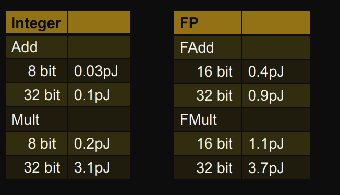 Energy Costs for various operations on a 45nm CMOS node. Source: Computing’s Energy Problem
So, integer arithmetic consumes lesser energy, specifically int8 add consumes 30x less energy than fp32 add & int8 mul consumes 18x less energy than fp32 mul. Lower precision hardware is also faster & consumes lesser silicon area than floating point.
How do these benefits translate to real-world gains? It depends on the bottleneck:
Compute-bound workloads (e.g., CNNs, LLM prefill): Quantization can improve throughput since lower-precision arithmetic is faster and consumes lesser energy.
Memory-bandwidth-bound workloads (e.g., LLM decoding): Quantization reduces the amount of data moved, improving performance by lowering memory bandwidth pressure.
By this point, the motivation should be clear: quantization reduces memory, lowers energy consumption, and can improve performance. Next, we will look at the hardware unit that executes fixed point arthmetic.
The dominant operation in neural networks is matrix multiplication. Modern hardware accelerators optimize this using specialized units called Multiply–Accumulate (MAC) Units:
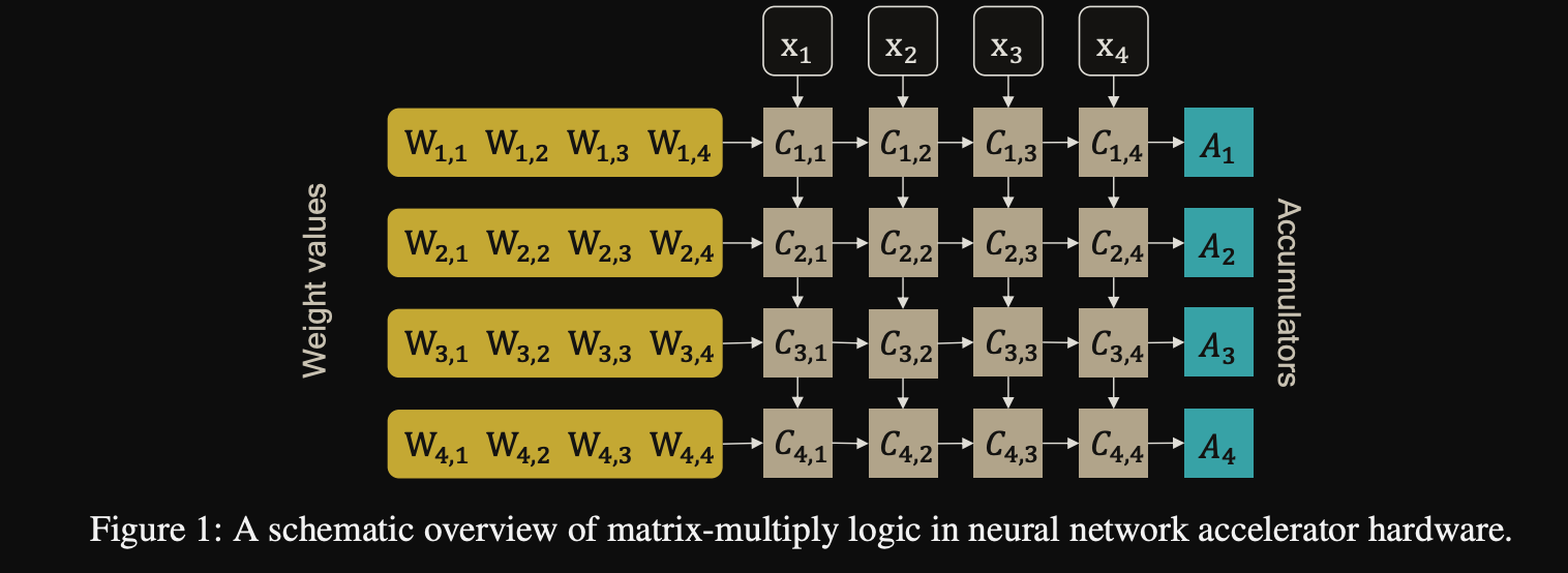
Matrix–vector computation in neural network accelerator hardware. Source: A White Paper on Neural Network Quantization
The diagram represents a typical matrix–vector multiply unit in neural network accelerators. This is the building block for matrix multiplications and convolutions. The two fundamental components are the processing elements \(C_{n,m}\) and the accumulators \(A_n\).
The computation proceeds as follows:
The accumulators are first initialized with the bias value \(b_n\)
In the next cycle, weights \(W_{n,m}\) and input values \(x_m\) are loaded
Their product is computed at each processing element:
$$C_{n,m} = W_{n,m} \cdot x_m$$
The results are then accumulated:
$$A_n = b_n + \sum_{m} C_{n,m}$$
Starting from a real-valued vector \(x\), we map it to an integer grid \(\{x_{\text{int}}^{\min}, \ldots, x_{\text{int}}^{\max}\}\):
$$ x_{\text{int}} = \mathrm{clamp} \left( \left\lfloor \frac{x}{s} \right\rceil + z,\; x_{\text{int}}^{\min},\; x_{\text{int}}^{\max} \right) $$
Here:
\(s\) is the scale
\(z\) is the zero-point (offset)
\(\lfloor \cdot \rceil\) denotes rounding to the nearest integer
The clamp operation ensures the result lies within the valid integer range:
So, the idea is to scale and shift the floating-point value, then clamp it to fit within the integer grid.
Instead of running quantized models directly on target hardware, we often simulate quantization on general-purpose hardware using high-level frameworks like PyTorch. This is commonly referred to as fake quantization.
The key idea is simple: we mimic the effects of quantization while still executing operations in floating point. This allows us to study accuracy and perform experiments like Quantization Aware Training (QAT) without requiring specialized hardware.
To do this, we:
The dequantization step maps integers back to real values:
$$ \widehat{\mathbf{x}} = s \left( \mathbf{x}_{\text{int}} - z \right) $$
Combining quantization and dequantization, we get:
$$ \widehat{\mathbf{x}} = q(\mathbf{x}; s, z) = s \left[ \mathrm{clamp} \left( \left\lfloor \frac{\mathbf{x}}{s} \right\rceil + z,\; x_{\text{int}}^{\min},\; x_{\text{int}}^{\max} \right) - z \right] $$
In practice, frameworks insert these quant–dequant (Q/DQ) pairs around operations in the model graph. While the computation is still carried out in floating point, the values are constrained to a discrete set, effectively simulating quantization effects during inference.
At this point, it’ll be helpful to build some intuition around what the quantization formula is actually doing.
Think about the minimum value that can come out of the quantization operation.
This corresponds to \(x_{\text{int}}^{\min}\). Plugging this into the de-quantization formula:
$$ q_{\min} = s \left( x_{\text{int}}^{\min} - z \right) $$
Similarly, the maximum value corresponds to \(x_{\text{int}}^{\max}\):
$$ q_{\max} = s \left( x_{\text{int}}^{\max} - z \right) $$
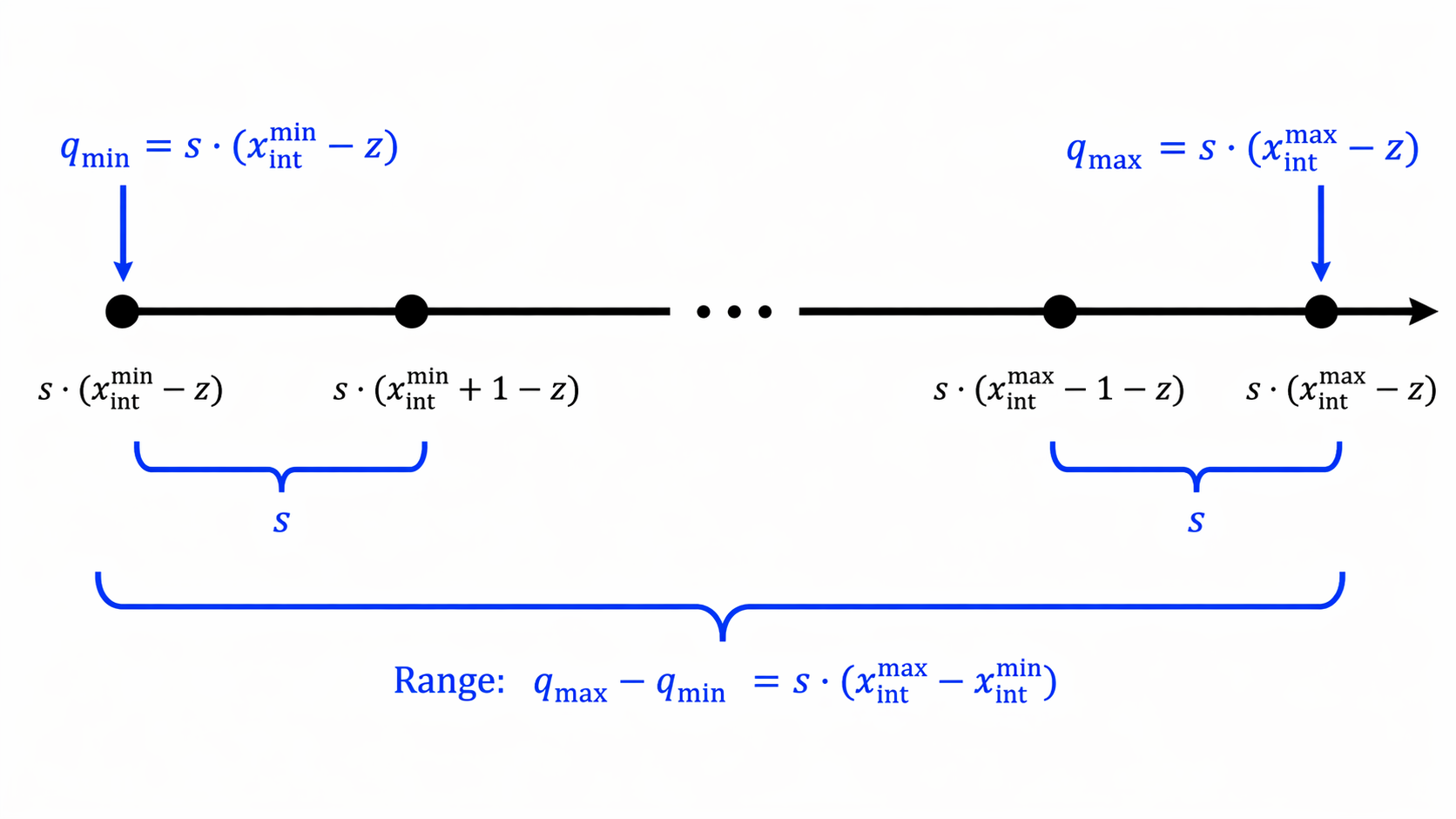
Key thing to note here is: we no longer operate over a continuous floating-point range, but over a discrete set of \(2^b\) values, each separated by the scale \(s\).
There are two “bad guys” in our quantization formula:
(1) the rounding operator, which introduces rounding error, and
(2) the clamp operator, which introduces clipping error.
These are the reasons why a quantized network deviates from the original network, a.k.a: quantization error (or quantization noise). As we’ll see, improving one often worsens the other, so quantization is really about balancing the two.
Rounding Error: for a value is the difference between the original floating-point value and the value it gets mapped to on the quantized grid.
Clipping Error: occurs when values fall outside the representable range and get clipped to the minimum or maximum value.
Let’s think about the extremes again. When would the rounding error be the maximum? The worst case occurs when the fp value lies exactly halfway between two grid points. In this case:
$$ \text{max rounding error} = \frac{s}{2} $$
So, you might think: “why not make \(s\) very small to minimize this for each value?”. Unfortunately, there’s no free lunch when it comes to quantization: reducing s makes [\(q_{\min} = s \left( x_{\text{int}}^{\min} - z \right)\), \(q_{\max} = s \left( x_{\text{int}}^{\max} - z \right)\)] smaller increasing your clipping error.
So how do you choose quantization parameters optimally?
The simplest approach is min–max quantization, where we use an unsigned integer grid \((0 \text{ to } 2^b - 1)\) and set the scale so that the entire floating-point range fits within it, avoiding clipping. That is, you want:
\(q_{\max}\) to map to \(fp_{\max}\) & \(q_{\min}\) to map to \(fp_{\min}\)
So you solve:
$$ q_{\max} = s \left(2^b - 1 - z\right) = fp_{\max} $$
$$ q_{\min} = -s z = fp_{\min} $$
Solving these gives:
$$ s = \frac{fp_{\max} - fp_{\min}}{2^b - 1} $$
$$ z = \frac{fp_{\min} \cdot (2^b - 1)}{fp_{\min} - fp_{\max}} $$
For a signed grid \((-2^{b-1} \text{ to } 2^{b-1} - 1)\), the corresponding method is abs-max quantization, where we scale using the maximum absolute value so that the range is symmetric around zero, avoiding clipping.
So you solve:
$$ q_{\max} = s \cdot (2^{b-1} - 1) = \max\left( |fp_{\min}|,\; |fp_{\max}| \right) $$
Solving gives:
$$ s = \frac{\max\left( |fp_{\min}|,\; |fp_{\max}| \right)}{2^{b-1} - 1} $$
$$ z = 0 $$
These are the most common formulas for scale and offset on the internet – now you known where they come from!
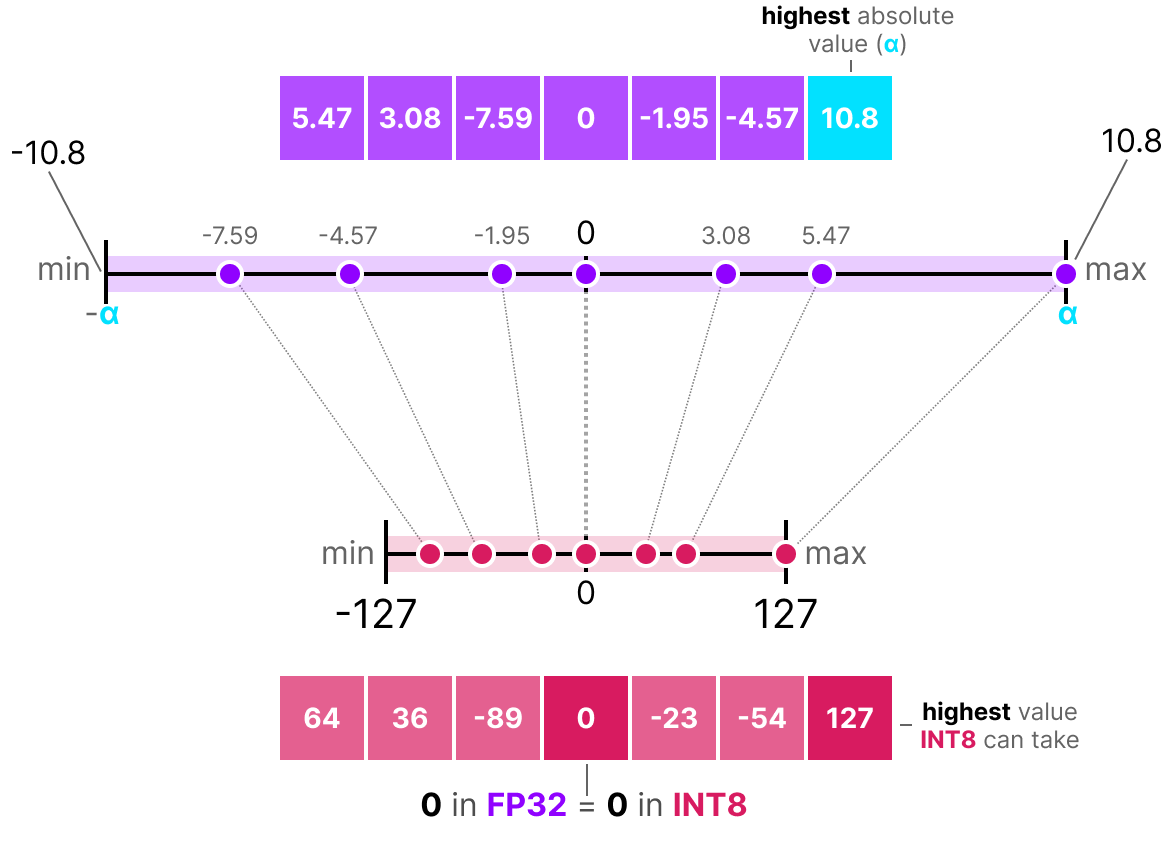 An example of AbsMax Quantization. Author Maarten Grootendorst
Notice how some of values in integer grid get wasted with AbsMax Quantization.
But what if your tensor contains outliers - i.e., a very small fraction of values have large magnitudes while most are relatively small?
If you use min–max or abs-max quantization, these outliers stretch the range of the grid. As a result, most values get mapped to a coarser grid, leading to higher rounding error.
Fortunately, there are alternatives:
Loss-aware quantization:
Choose the quantization parameters (e.g., range, scale) to minimize a loss between the floating-point and quantized outputs - such as MSE, cross-entropy, or SQNR.
Range clipping:
Instead of covering the full range, clip extreme values (e.g., using percentiles) to reduce the impact of outliers and improve effective resolution.
Even these do not guarentee that quantization will work well but thankfully we have a few more axes to play with. And that’s exactly what we’ll explore next.
Quantization can be divided based on :
Affine (asymmetric) quantization uses a non-zero zero-point \(z\), allowing the quantized range to better align with the floating-point distribution. It is commonly used with unsigned integer grids and provides flexibility by shifting where real zero is represented.
In contrast, symmetric quantization enforces \(z = 0\), using a range centered around zero. It is typically paired with signed integer grids and works well when the data distribution is approximately zero-centered.
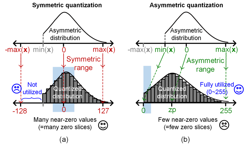
Let’s see how this choice affects computation.
Recall:
$$ A_n = b_n + \sum_m (W_{n,m} \cdot x_m) $$
When \(W_{n,m}\) and \(x_m\) are quantized:
$$ W = s_w (W_{\text{int}} - z_w), \qquad x = s_x (x_{\text{int}} - z_x) $$
Substituing, we get:
 Source: A White Paper On Neural Network Quantization
The first term matches the symmetric case.
The third and fourth terms depend only on weights, scales, and offsets, so they can be precomputed and folded into the bias at negligible cost.
The second term, however, depends on the input \(x\), meaning it must be computed at inference time, adding latency and power overhead.
Hence, a common strategy is asymmetric activations + symmetric weights, which avoids this data-dependent cost.
One entire tensor shares a single scale (\(s\)) and zero-point (\(z\)).
Effective bits per value:
Assuming the scale and zero-point are stored in 16 bits each, the effective number of bits per value is:
$$ \text{effective bits} = b + \frac{16 + 16}{N} $$
where:
Example:
For \(N = 1024\) and \(b = 8\):
$$ \text{effective bits} = 8 + \frac{32}{1024} = 8.03125 $$
So, 8-bit quantization requires slightly more than 8 bits per value once the scale and zero-point are included.
Each channel has its own scale (\(s\)) and zero-point (\(z\)).
Assume a matrix of shape \((C, K)\), where each row (or column) is a channel.
Effective bits per value:
$$ \text{effective bits} = b + \frac{C \cdot (16 + 16)}{N} $$
where:
Example:
For a matrix with \(C = 64\) channels and \(K = 16\) values per channel:
$$ N = 64 \cdot 16 = 1024 $$
$$ \text{effective bits} = 8 + \frac{64 \cdot 32}{1024} = 10 $$
A block of values shares a single scale (\(s\)) and zero-point (\(z\)).
Effective bits per value:
$$ \text{effective bits} = b + \frac{16 + 16}{B} $$
where:
Example:
For a block size of \(B = 64\) and \(b = 8\):
$$ \text{effective bits} = 8 + \frac{32}{64} = 8.5 $$
In general, finer-grained schemes (more parameters) yield better accuracy but introduce additional storage and compute overhead. Per-channel quantization generally offers a good tradeoff for weights, while per-block quantization is applied to particularly sensitive weights. However, per-channel quantization for activations is hardware-inefficient and the reason becomes clear once you expand the MAC computation.
With per-channel quantization, weights and activations each have their own per-channel scale vectors:
$$ \mathbf{s}_w = [s_{w_1}, s_{w_2}, \ldots, s_{w_n}], \qquad \mathbf{s}_x = [s_{x_1}, s_{x_2}, \ldots, s_{x_m}] $$
Substituting the dequantized values into the accumulator equation:
$$ A_n = b_n + \sum_{m} \left( W_{n,m} \cdot s_{w_n} \right) \cdot \left( x_m \cdot s_{x_m} \right) $$
$$ A_n = b_n + s_{w_n} \sum_{m} W_{n,m} \cdot x_m \cdot s_{x_m} $$
Notice that \(s_{w_n}\) does not depend on \(m\), so it can be factored out of the summation and applied as a single scalar multiply after accumulation. This is cheap and hardware-friendly. \(s_{x_m}\), however, depends on \(m\) which means it cannot be factored out. Instead, each product \(W_{n,m} \cdot x_m\) must be rescaled by a different \(s_{x_m}\) before accumulation. This is why per-channel quantization is standard for weights but avoided for activations.
Since weights are always known before inference they can be quantized offline, however, activations depend on the input to the model, and there are two ways of quantizing them.
In static quantization, the min and max ranges of activations are calculated using a small subset of the training data called calibration dataset which typically contains around 300-500 samples.
In dynamic quantization, the min-max ranges are calculated on the fly during inference. This is useful in situations where the model execution time is dominated by loading weights from memory rather than computing the matrix multiplications.
For integer quantization, static quantization is most common.
Quantization aware training (QAT) simlutes inference-time quantization duering training by using quantized weights and activations in the forward pass, while using full precision weights in the backward pass. The idea is to emulate the inference time quantization error by using quantized values in the forward pass, and allowing the backward pass to update the full-precision weights such that they become more robust to quantization. This approach leads to better accuracy preservation as the model learns to adapt to the precision loss during training.
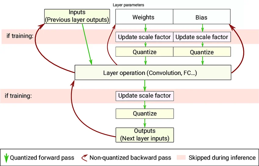
Quantization Aware Training. Source: Quantization and Deployment of Deep Neural Networks on Microcontrollers
Unlike quantization aware training, where the model learns to adjust to lower precision during training, post-training quantization (PTQ) directly applies this reduction in bit width after the model has been trained. While it may not offer the same level of accuracy preservation as quantization aware training, it is widely used in practice since it doesn’t require retraining the model.
In this series, we will primarily focus on post-training quantization (PTQ) techniques.
The weights and activations are loaded in low precision (e.g., int8 × int8, or int8 × int16 on some hardware). Since inputs are quantized, we move less data. Each cycle performs the multiply (e.g., 8×8 or 8×16), and the results are accumulated in higher precision, typically int32.
So does the next layer receive 32-bit values? Not quite. We requantize the accumulator back to low precision before passing it on.
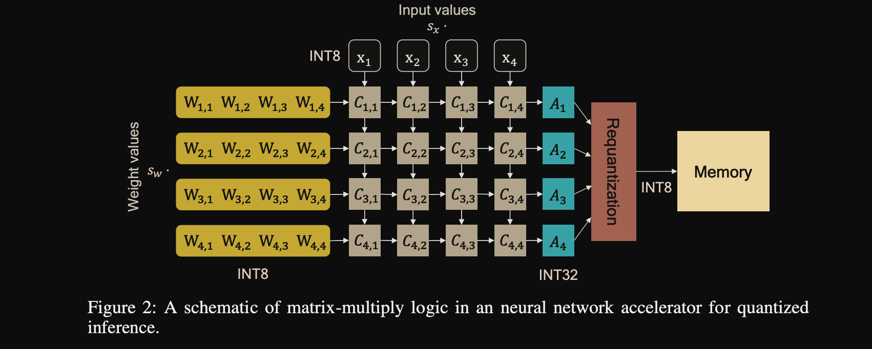
Source: A White Paper On Neural Network Quantization
Recall that on the MAC, the accumulator computes:
$$ A_n = b_n + \sum_{m} C_{n,m} = b_n + \sum_{m} W_{n,m} \cdot x_m $$
When weights and activations are quantized, the real values are recovered via dequantization:
$$ W_{n,m} = s_w \left( W_{\text{int}_{n,m}} - z_w \right), \qquad x_m = s_x \left( x_{\text{int}_m} - z_x \right) $$
Substituting into the accumulator:
$$ A_n = b_n + \sum_{m} s_w \left( W_{\text{int}_{n,m}} - z_w \right) \cdot s_x \left( x_{\text{int}_m} - z_x \right) $$
$$ A_n = b_n + s_w s_x \sum_{m} \left( W_{\text{int}_{n,m}} - z_w \right)\left( x_{\text{int}_m} - z_x \right) $$
The hardware computes the inner sum entirely in integer arithmetic, accumulating into a high-precision int32 register:
$$ A_{\text{int}_n} = \sum_{m} \left( W_{\text{int}_{n,m}} - z_w \right)\left( x_{\text{int}_m} - z_x \right) $$
So the real-valued accumulator output is simply:
$$ A_n \approx s_w s_x \cdot A_{\text{int}_n} $$
Now, this output needs to be passed to the next layer which expects quantized inputs with its own scale \(s_y\) and zero-point \(z_y\). So we need to quantize \(A_n\):
$$ y_{\text{int}_n} = \left\lfloor \frac{A_n}{s_y} \right\rceil + z_y = \left\lfloor \frac{s_w s_x}{s_y} \cdot A_{\text{int}_n} \right\rceil + z_y $$
Defining the requantization scale:
$$ M = \frac{s_w s_x}{s_y} $$
The full requantization step becomes:
$$ y_{\text{int}_n} = \mathrm{clamp}\!\left( \left\lfloor M \cdot A_{\text{int}_n} \right\rceil + z_y,\ y_{\text{int}}^{\min},\ y_{\text{int}}^{\max} \right) $$
This is the only floating-point operation in the pipeline - multiplying the int32 accumulator by \(M\) to rescale it into the next layer’s quantization range.
In practice, \(M\) is implemented using fixed-point arithmetic (an integer multiply followed by a bit shift), keeping the entire pipeline in integer arithmetic - see Quantization and Training of Neural Networks for Efficient Integer-Arithmetic-Only Inference , Section 2.2, for the full derivation.
That was a lot to cover and, if you made it this far, well done! We looked at why quantization matters (memory, energy, throughput), how it works mathematically (the quantization and dequantization pipeline, rounding vs clipping tradeoff), the key design choices (symmetric vs asymmetric, per-tensor vs per-channel vs per-block, static vs dynamic, PTQ vs QAT), and why certain combinations like symmetric weights with asymmetric activations, or per-tensor activation quantization are preferred in practice.
All of this assumes the weight and activation distributions are reasonably well-behaved. In the next post, we’ll see why transformers break that assumption and why that makes quantizing them surprisingly hard.
此内容由惯性聚合(RSS阅读器)自动聚合整理,仅供阅读参考。 原文来自 — 版权归原作者所有。