Sharing a visualization from a Datadog dashboard or notebook is simple. You can copy and paste a widget directly into another dashboard, message, or document. Behind the scenes, the widget is stored with a unique sharing URL, which the Datadog app or chat integrations can use to render a live preview or link back to the underlying data.

These live previews are especially powerful when using Datadog Incident Management’s docked view. When an incident is docked, pasting a widget into a Slack incident channel renders it as a fully interactive widget in Datadog, letting users correlate key indicators from an incident with other metrics during investigation and remediation.

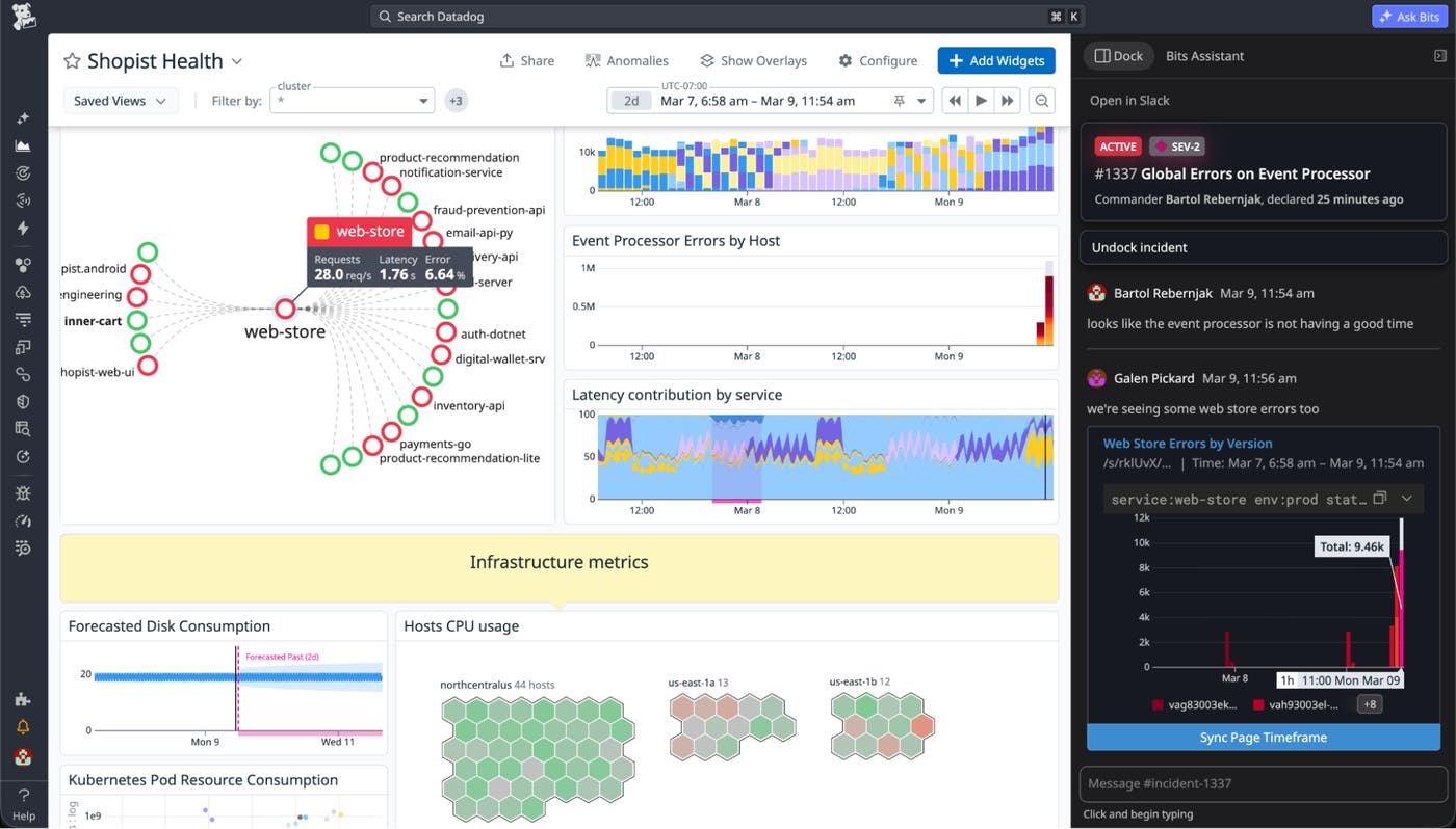
Although this feature captures full context for visualizations, many users still prefer to take screenshots.

Screenshots are quick, intuitive, and guarantee a consistent visual snapshot, regardless of context or permissions. However, taking screenshots loses a lot of valuable information, such as the time range, underlying query, visualization type, and the dashboard state at the moment the image was taken.

This led us to a question: What if screenshots could carry the same context as share links, without changing how they look?

In this post, we’ll show you how we built a system to invisibly embed widget metadata inside a screenshot using a pixel-level encoding scheme. We’ll cover:

• How we compress, encode, and render metadata without affecting the user experience

• Why we needed to build resilient watermarking that survives color profiles, display densities, and copy-paste workflows

• The backend systems we use to cache and retrieve this metadata

• Performance optimizations that let us render over a billion watermarks per day without impacting app responsiveness

Along the way, we’ll share what worked, what didn’t, and how we balanced scale, resilience, and invisibility to build a feature that’s always on, but only noticeable when you need it.

How it works today

When you copy a widget in Datadog, we generate a backend record containing the widget definition and store a reference to it in your clipboard as a share URL. Pasting this URL into another dashboard or notebook restores the original widget. If you paste the URL into Slack or Teams, the Datadog chat integration displays a preview of the graph and its title:

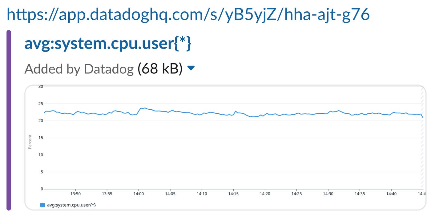
Clicking the link opens the original widget in Graph Explorer, preserving time range, queries, and other configuration details.

Could we make these features work even if you take a screenshot instead of copying the widget? The question came up in one of our internal engineering channels.

More than a dozen engineers from teams across the company chimed in, sharing thoughts on the problem and ideas for a solution. Throughout the discussion, we explored existing approaches to similar problems and a handful of original ideas. Eventually, we landed on something that sounded promising: watermarking.

We wanted a way to embed metadata in a screenshot without affecting the user experience or adding more UI elements to an already crowded dashboard. Maybe we could subtly alter the colors of some pixels inside a widget—invisible to the naked eye, but recoverable by a watermark-reading algorithm.

How much data can we even encode in a watermark?

Widget definitions can be deceptively large. They include all the data requests and queries, display settings, legend configuration, time frame overrides (if present), and the title. If the widget comes from a dashboard, we also want to include the current time frame, template variable values, widget dimensions, and a deep link.

On average, this adds up to around 2 kB per widget. That is a lot of data to encode in a nearly invisible image, especially when it needs to work reliably even for the smallest widgets.

Encoding just enough data

Instead of encoding entire widget definitions, we write them in a Redis cache. Each record contains a full widget definition, stored behind a randomly generated key. That key—a fraction of the record’s size—can be encoded into a watermark.

Widget definitions contain a snapshot of the widget’s current state. So if the widget’s data is refetched, the time frame changes slightly, or its definition is updated, we generate a new snapshot, cache it, and embed a new watermark.

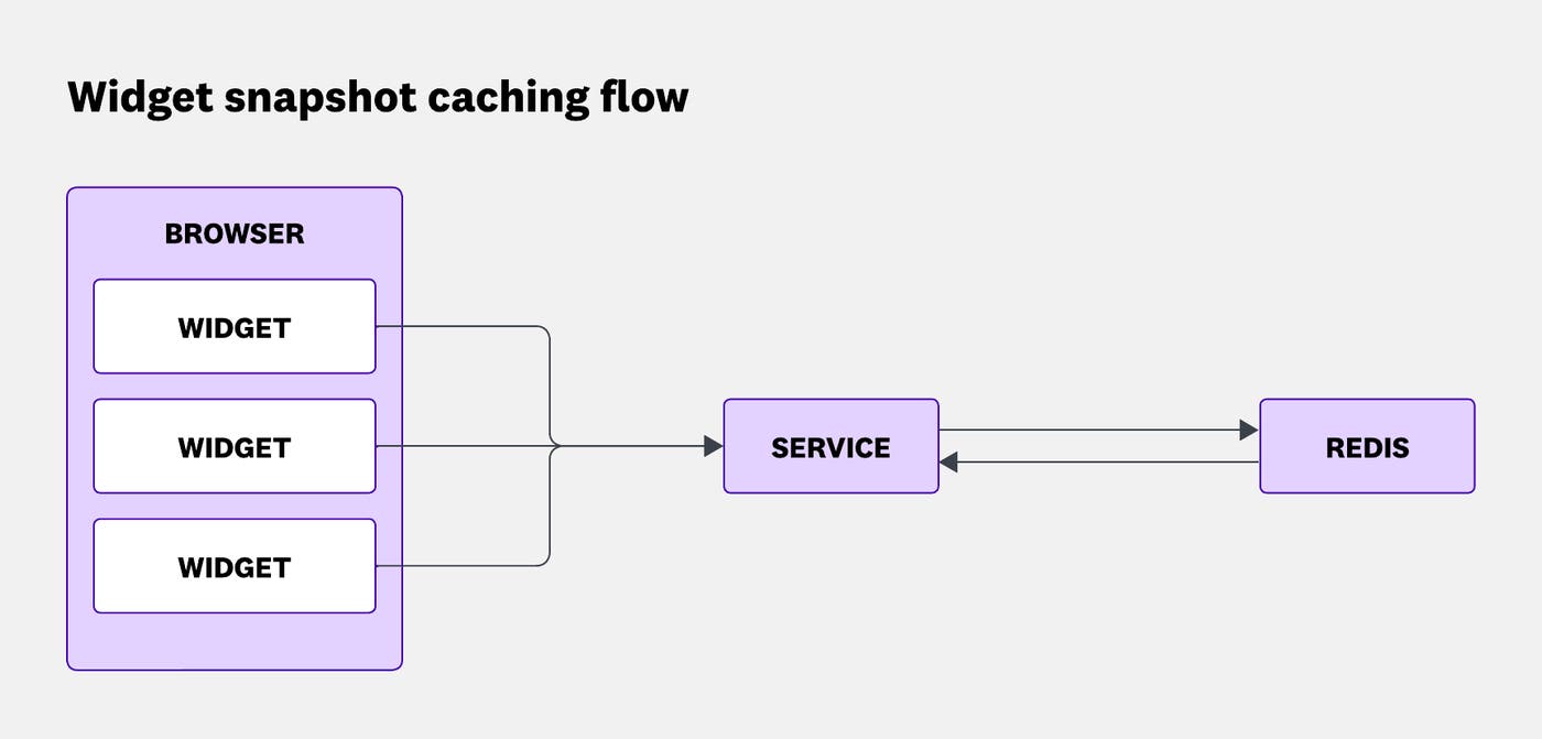
To ensure that watermarks are displayed as soon as widgets are rendered, we generate the snapshot ID optimistically on the frontend before the record is actually cached. This avoids waiting for the service response, but introduces a small risk of ID collisions.

How small? Across all production data centers, we render just over 1 billion widgets per day, with peaks around 125 million widgets per hour (about 35,000 per second). Most screenshots are taken and pasted within a few seconds, and almost never more than a few minutes later. So we keep all snapshot records cached for one hour, allowing us to detect and recover watermarks from recently rendered widgets.

Smaller IDs are easier to hide invisibly in an image, but at that scale, small IDs introduce a non-trivial collision risk. The risk of two of your widgets receiving the same ID needs to be small, but the risk of one of your widgets receiving the same ID as a widget from another Datadog customer needs to be zero. To guarantee this, we construct our Redis cache key by prepending an organization ID to the widget ID.

No single customer accounts for more than 1% of our widget renders, so we can use 1 million IDs per hour as a reasonable upper bound. 1 million IDs means 5×10¹¹ ID pairs, and an 8-byte ID gives us 2⁶⁴ ≈ 1.8×10¹⁹ possible values. Dividing these two numbers gives us an approximate probability of collision: roughly 1 in 37 million.

But how do we invisibly embed 8 bytes of data into a dashboard widget?

Every dashboard widget has a thin, 1 px border of a uniform color. While the widget contents vary a lot depending on the chosen visualization and configuration, the border is always there. That made it an ideal place to embed the watermark without having to implement any visualization-specific logic.

Our first idea was simple: Line the top or the bottom border (they are usually longer than side borders) with pixels in two different colors, each representing a single bit.

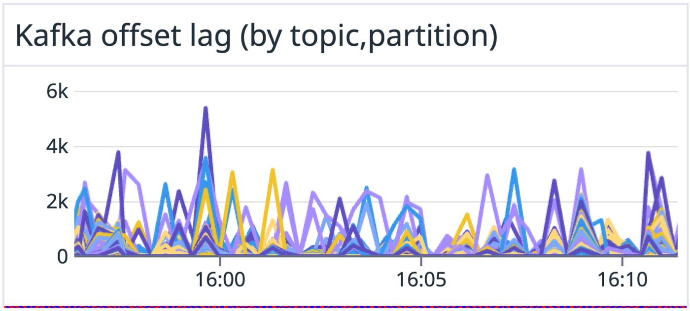
Unfortunately, for 8 bytes of data, this would require at least 64 pixels. While our smallest widget is still wider than that, the larger the watermark, the more likely it is to be visible to the eye, even if we use colors similar to the base border color instead of bright red and blue. We wanted smaller watermarks, ideally no longer than 10 pixels. Could we store an entire byte in a pixel?

In the RGB model, each pixel has three color channels. This gave us an opportunity: We split a byte of data into three values and use them to offset the base RGB values of the border, encoding our data directly into the image.

Given a background RGB color, we calculate the base color by subtracting 3 from each channel. Then we increase the values by up to 7, to store up to 9 bits per pixel. For example, increasing R by 5, G by 7, and B by 1, encodes 101-111-001 in bits.

To mark the watermark region, we use two sentinel pixels at the start and the end, encoded as +7/7/7 per RGB channel (111-111-111). So if the base color is #e0e0e0, the sentinel pixels become #e7e7e7.

The eight pixels between those sentinels each store one byte of data, using three bits from the R, three from the G, and the top two bits of the B channel.

This is what that layout looks like:

Below is a screenshot of a watermark generated using this method, placed along the top border of a dashboard widget, zoomed in at 8,000%.

The color profile problem

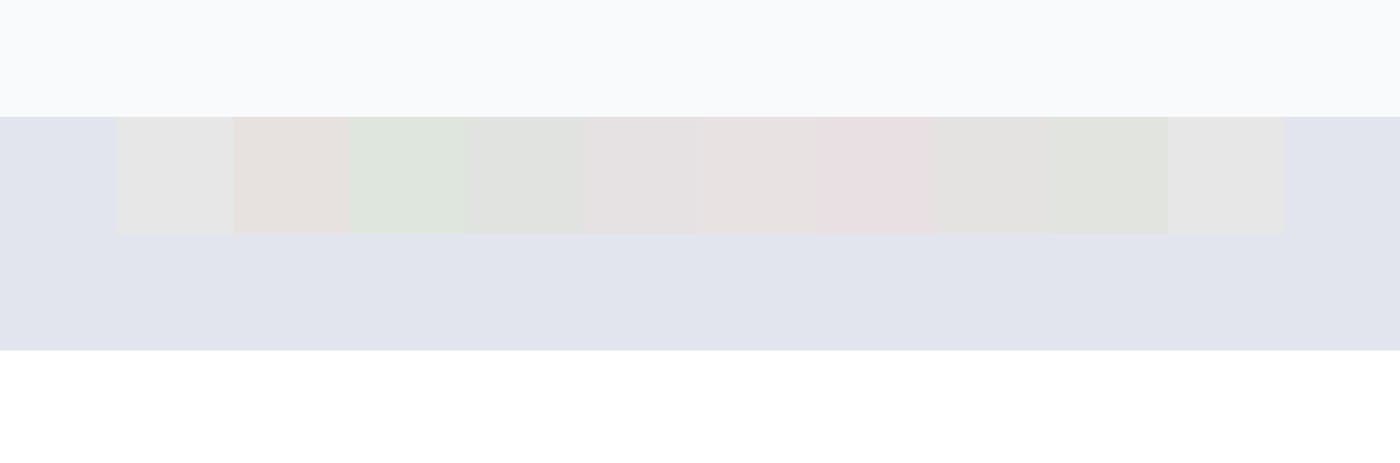
At this point, you might notice a problem with our approach. It would work perfectly, if everyone only used RGB displays.

When we generate a watermark using RGB color values and take a screenshot on an RGB device, we can recover the exact original colors from the image. But many modern displays use other color profiles.

For example, taking a screenshot on a DCI-P3 device (like a Retina MacBook) and converting it back to RGB often shifts some channel values by ±1. The values don’t map properly, and we’re left with ambiguous decimal values that are hard to interpret. For an encoding scheme that relies on exact color values, that’s a deal breaker.

Also, depending on the ID, the watermark was sometimes visible. A casual user wouldn’t notice it, but if you knew where to look, you could spot it. That told us we should decrease the color variance, even if it meant using more pixels.

Solving the color gamut problem with fuzzy encoding

Third time’s a charm.

To make the watermark resilient across different color gamuts, we switched to a fuzzy encoding approach. By mapping each part of the ID to a range of neighboring colors, we could still recover the original value, even if the colors are slightly offset.

With this method, each pixel stores just 2 bits of data. This gives us a short enough watermark (34 pixels wide), while reducing the number of colors needed. Fewer colors means we stay closer to the base color, making the watermark significantly less noticeable.

Given a background RGB color, we could encode up to 2 bits per pixel—one in the red channel and one in the green—by offsetting the base color. During watermark generation, a +3 offset encodes a 1 and -3 encodes a 0. When decoding, offsets in the range of [+1, +5] are interpreted as 1, [-1, -5] as 0, and anything in (-1, 1) as undefined. The blue channel doesn’t carry data but helps distinguish sentinel pixels from data pixels: a valid sentinel has red and green offsets within [–1, 1] and a blue offset within [+1, +5].

As an example, let’s take (226, 229, 237) as our base color. This is the actual border color for dashboard widgets. A base pixel would look like this:

To designate a pixel as a sentinel pixel, which would mark the beginning of a watermark, we would shift that color by +0/+0/+3, resulting in a slightly more blue (226, 229, 240) pixel:

Let’s try encoding 10110011, a single byte of data. This would be split into four pixels, two bits per pixel: +3/-3/+0, +3/+3/+0, -3/-3/+0, +3/+3/+0. This results in (229, 226, 237), (229, 231, 237), (223, 226, 237), and (229, 232, 237):

Drawing that on top of our background color, wrapped with a sentinel pixel on both sides, gives us this:

You might say it’s pretty visible, but keep in mind this is scaled up about 80x.

We can take this through any color gamut remapping and be sure that converting it back to RGB will keep the values within the same ranges, allowing us to read the originally encoded value.

More tuning for real-world screenshots

At this point, we had a resilient encoding method.

Does that mean our watermark could be picked up reliably from screenshots in any situation? Nope.

During internal testing, we used RUM to find Datadog employees with unusual setups—devices with uncommon screen densities, operating systems, or browsers:

(@usr.is_datadog_employee:true @session.type:user
(-@context.screen.pixel_ratio:1 -@context.screen.pixel_ratio:2) OR
-@os.name:"Mac OS X" OR -@browser.name:Chrome)

We asked them for dashboard screenshots, and their screenshots made clear that our work wasn’t done yet.

Handling different pixel densities

Remember the 1 px dashboard border we mentioned earlier? On one of our screens, it actually takes up 2 px, and it shows up as 2 px thick in the screenshot. Why?

There are a lot of devices browsing the web today. Somewhere out there, someone is still using a 1024x768 CRT monitor from the early 1990s. Someone else is using a 23-million-pixel Apple Vision Pro headset from 2024. The most commonly used unit for laying out web pages is still the CSS pixel. But to make sites look consistent across devices, browsers scale those pixels depending on the screen’s pixel density. This scale is called Device Pixel Ratio (DPR).

On a standard 1920x1080 screen, DPR is 1. On higher-resolution displays (like 14” MacBook Pro), it’s often 2. Some phones even hit 3.

If you specify a CSS width of 100px, it will render as 200 physical pixels on a DPR 2 screen.

Fun fact: DPR is what changes when you zoom in and out with cmd/ctrl + scroll.

To keep the watermark easy to read, we always want it to be exactly one physical pixel tall and 34 pixels wide. On high-DPI screens, this makes it smaller and even less visible. On lower-density displays, it might be more noticeable, but we cannot scale it down without making it unreadable.

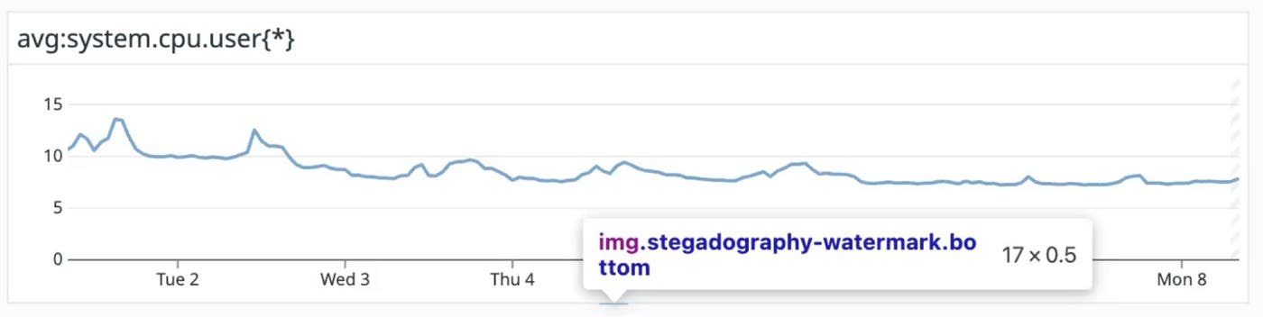
In code, this is simple: there’s a global devicePixelRatio value on the window object. We just set the watermark’s height to 1/DPR pixels. In Chrome DevTools, the watermark shows up as 0.5 px tall.

But when we take a screenshot? It is exactly 1 px tall.

Further optimizations

Ultimately, an invisible feature that needs to be enabled all the time—but is useful only occasionally—should not affect overall performance. We don’t want to penalize users who never take screenshots by making their dashboards slower or less responsive.

So we spent some time on performance tuning and implemented a handful of optimizations to minimize overhead.

Choosing how to paint pixels

We tried and tested multiple methods of painting pixels.

An SVG made up of 1x1 rectangles was the easiest thing to generate dynamically in React, and it worked well in our initial prototype. But it has two major problems:

• It added n+1 DOM elements per watermark, where n is the number of pixels.

• With two watermarks per widget—and potentially dozens or hundreds of widgets on a dashboard—that’s a lot of DOM overhead.

On top of that, the CPU cost of rendering vector graphics to the screen’s raster added noticeable browser lag.

Surely there had to be a better solution.

Canvas rendering (better, but not great)

The obvious next step was canvas. Since canvas is based on a pixel grid, it’s much better suited for raster imaging.

We tried creating a small canvas for each watermark and drawing pixels with putImageData or fillRect. We also set imageSmoothingEnabled to ensure neighboring pixels didn’t blend together and lose their exact values.

We used feature flags and A/B tested this with RUM. The results were clear: Canvas was faster than SVG in real-world dashboard performance.

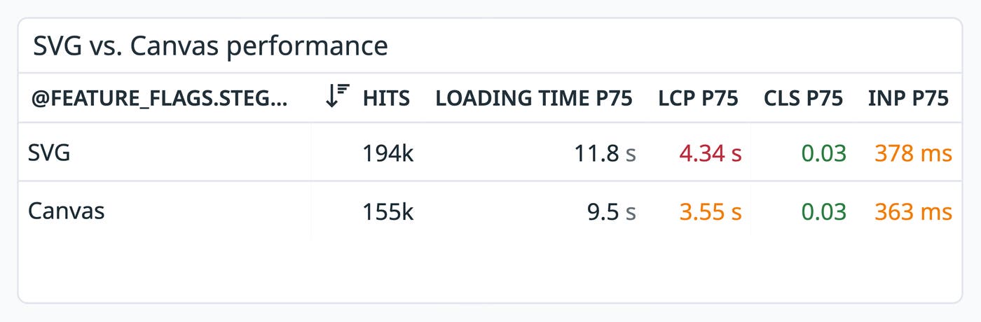
But it still felt like we were hogging too much CPU and memory just to paint a few pixels on the screen. Even using toDataURL("image/png") to export a canvas as an image would require creating a canvas we didn’t really need.

Generating the pixels ourselves

What if we skipped rendering altogether and just wrote the bytes ourselves?

We considered using a library like jimp to generate images directly, but it’s a pretty big dependency to ship just for a feature that’s meant to be invisible and low-cost.

Our watermarks are simple. How hard could it be to write a few colored pixels into a file?

We looked at the structure of a basic BMP file:

• BMP Header: Contains a hardcoded signature, file size, and byte offset to the pixel data.

• DIB Header: Contains header size, width, height, number of color planes (usually 1), bits per pixel, compression, resolution, size of the image data, and the optional color table.

• Pixel array: Contains pixel data. Based on the bits per pixel, the data is split into individual pixels, with each pixel’s color defined across the red, green, and blue channels.

There is a strong pattern across all the watermark images we generate:

• Same file size

• Same byte offset

• Same header values (size, width, height, number of bits per pixel, no compression, same resolution, and so on)

• Always 34 pixels

The only thing that changes is the pixel array itself, the RGB values.

After some tweaking, we settled on hardcoded headers. At runtime, we just fill in the rest of the file with bytes for the blue, green, and red channels (yes, in that order—BMP stores them BGR) and generate a Base64 BMP URL to use in the <img/> tag.

Watermarks are now generated with minimal time complexity: a single loop with 34 iterations appending bytes to an array, and a single btoa() call to turn it into a Base64 string.

Sending out caching requests

Remember, we want to create one billion watermarks per day. Every time a widget’s appearance changes for any reason, it’s a new watermark. Every visible watermark needs to reference an entry in the backend cache that contains the corresponding widget definition.

How do we get those definitions into the cache?

If we send out an AJAX request for every watermark, we risk impacting page performance. On a page as request-heavy as a dashboard, this can slow down essential data fetching and processing. We’d also prefer to minimize the number of requests our service receives and the number of cache calls.

We decided to batch the frontend request. Every time a widget is rendered, its watermark is added to the caching queue. Exactly three seconds after the first watermark is added to the queue, all queued entries are submitted to the caching endpoint. This introduces a subtle delay—at most three seconds—but doesn’t harm functionality.

If we are trying to detect widgets in an image and we don’t find any, it’s safe to assume they might just not have been cached yet. Retrying the same cache read five seconds later is usually enough to find any that were delayed.

These caching requests behave differently from most requests in our single-page app. We’re not fetching data to display or storing any user input. The user doesn’t directly care—nor know—whether the request was executed or whether it completed successfully. And neither does the app lifecycle. If the request fails, there’s nothing to do: no error message to show, no state to clean up or adjust.

With that in mind, we moved the request logic out of the React app’s lifecycle to avoid introducing unnecessary context. Instead, we set up a dedicated web worker to manage the queue and send caching requests. Because web workers run in a separate thread, we also off-loaded as many computational tasks as possible to avoid blocking the main JavaScript thread.

In the end, we built a React hook that any component can call with a widget definition. The hook passes the definition to the web worker, which adds it to the queue and generates the appropriate watermark. The only thing it returns to the calling component is the Base64 URL for the watermark bitmap. After all, that’s all the component needs.

Compressing large payloads

During extended testing, we noticed that some batch requests were quite large. For users quickly scrolling through a populated dashboard, the payloads could easily reach several hundred kilobytes and sometimes time out.

These batches are made up of similarly-shaped JSONs, sent from a web worker. They’re repetitive. And since we’re already inside a web worker, we can do some “cheap,” non-blocking computation.

It was time to do some gzipping in the browser.

We noticed that compressed requests were about 10x smaller than uncompressed ones, and the number of timeouts dropped by roughly 90%. We now compress any request that includes 10 or more widgets, about 35% of all requests. This avoids extra computation for small batches while ensuring large ones are compressed efficiently.

Deprioritizing off-screen content

The last optimization we made on the frontend is something we often did with widgets, both in the context of data fetching and rendering: deprioritizing off-screen content. We don’t render watermarks or cache widget contents if they are not visible, because they cannot be screenshotted anyway.

Supporting various color schemes

To keep the watermarks invisible, we want to use colors that are close to the base border color. This shouldn’t be hard, right? Dashboard widgets always use the same border color.

Ah—wait. There’s a dark theme. And high contrast, right. With different colors for both dark and light themes. That’s four different backgrounds so far?

Did you know notebooks use different colors, too? We do now, but we weren’t too happy when we found out.

Still, the frontend part is easy. We just pick a color based on the page and context. But how can the backend know what color to expect? In theory, we could explicitly support every possible color scheme, but that would require constant manual updates and would be fragile in practice, breaking anytime the frontend changes a theme or tweaks a color variable.

What if the backend just looks for any two pixels of the same color that are exactly 32 px apart? Those could be sentinel pixels. From there, we can infer the base color and check whether the pixels between them form a valid watermark for that color.

When you think about it, it’s just an extra short loop. Doesn’t add much complexity. But it adds a lot of flexibility.

We were pleasantly surprised to find out that even heavily tinted screenshots of widgets were still completely readable.

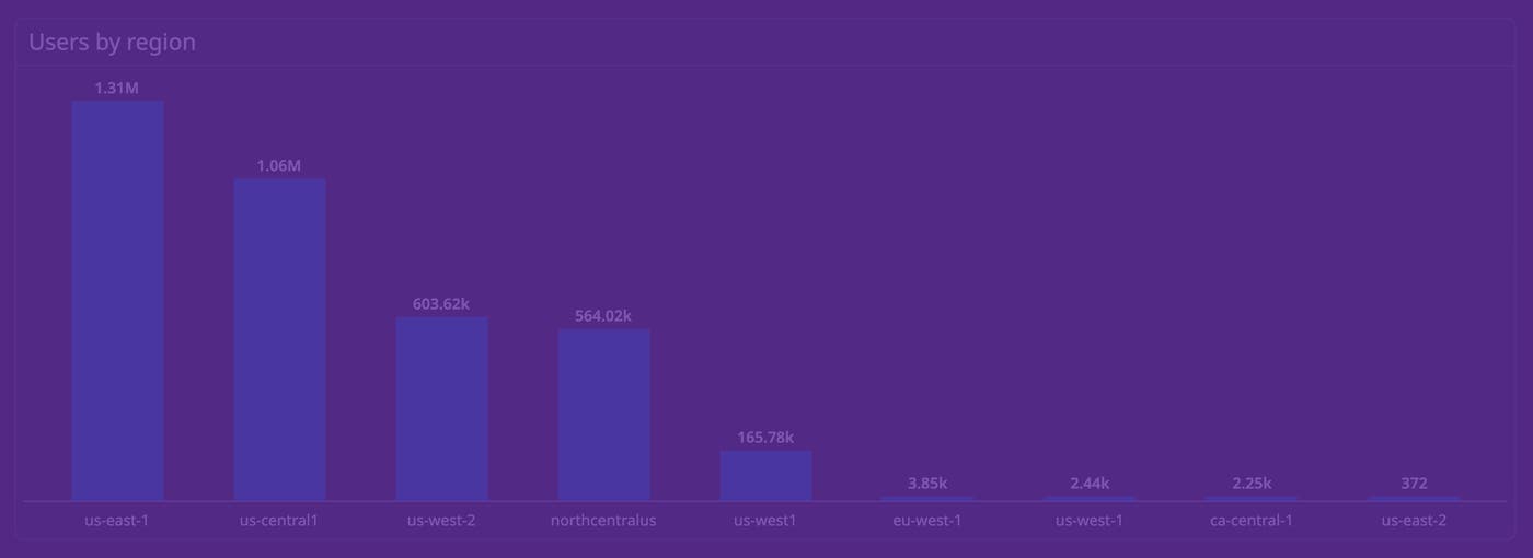
Detecting watermarks through color tint is a cool trick, but it’s not that useful.

The real win is that the frontend can dynamically pick a color that blends in, and the backend will still detect the watermark. There’s no need to hardcode values for every specific context. That makes it possible to place watermarks in even more places, including UI elements that change color dynamically or unpredictably.

Possible applications

We can take this further.

Because screenshots now carry recoverable metadata, they don’t have to be static artifacts anymore. Today, you can paste a widget screenshot directly into a dashboard and reconstruct it as a fully functional visualization.

This opens up new ways to move between visual context and live data without changing how users share or capture information today.

In addition to reconstructing widgets from screenshots, there’s also that Slack integration we mentioned earlier. We could convert screenshots into practical sharing links and attach them to the messages that contain screenshots, just like we already do when you paste a share link and we add a snapshot.

This would make chat history a lot more useful, since sharing links live forever and watermark definitions expire after an hour.

Wrapping up

We built a system that embeds widget metadata invisibly inside screenshots—resilient to color profiles, DPI settings, and even copy-paste workflows.

It runs constantly, adds no visual noise, and can generate over a billion watermarks per day without slowing anything down. The result is a feature that’s nearly impossible to notice until the moment you need it.

If solving hard frontend performance problems at scale sounds like your kind of challenge, we’re hiring!