





Without experiment infrastructure to help you test your LLM applications, every research session starts with the same questions: What have we tried previously? What were the numbers? Which prompt version produced that result? Why did we discard that approach? The answers live in scattered notes, terminal history, and half-remembered conversations. Each handoff between sessions loses context. In practice, iteration can slow down as teams get bogged down in testing and analysis.
The Datadog team responsible for building and maintaining Database Monitoring (DBM) needed to tackle these challenges in order to explore whether an AI agent could augment DBM’s automated query optimization recommendations. The DBM team used Karpathy’s autoresearch tool to trigger 23 autonomous experiments that brought the query optimization recommendation agent from precision scores of P=0.54 to P=0.86 overnight. Through this iterative process, the team proceeded through three phases:
Optimizing the prompt and tool chain
Rightsizing the model for an appropriate cost-performance tradeoff
Breaking the LLM call into two separate passes to break through a final performance barrier
In this post, we’ll discuss the autoresearch-powered experimentation process in depth, exploring how the team planned and executed rapid iteration of the agent by using LLM Observability Experiments to track, analyze, and act on the experiment results.
DBM’s query optimization recommender currently uses a multi-source heuristic engine (written in Go) that combines SQL parse-tree analysis, real explain plans, schema metadata, and runtime metrics to detect optimization opportunities. It covers six pattern families:
Missing index detection with plan-flip analysis (detects when the planner alternates between strategies)
SELECT * expansion with schema-aware column enumeration
ORDER BY without LIMIT with metrics-based row-count thresholds
OFFSET without ORDER BY (pagination correctness)
Idle-in-transaction detection via activity event analysis
Comprehensive SQL rewrite rules (OR to ANY, CAST normalization, date-to-range, CTE filter pushdown, and more)
This engine is precise by design. Each pattern is validated against actual database context. Explain plans use relative cost filtering. Metrics-based scoring avoids false positives on small result sets. On our evaluation dataset, it achieves a precision score P=0.903.
The DBM team wanted to see if an AI agent could run after the heuristic engine to discover additional optimization patterns. They hypothesized that an agent could discover types of patterns that are harder to encode as individual heuristic rules because they require cross-referencing multiple signals or understanding subtle semantic tradeoffs. For example:
A sequential scan on an indexed column might mean stale statistics (needs ANALYZE), not a missing index.
A covering index exists but is not being used as an index-only scan, suggesting a stale visibility map (needs VACUUM).
An expensive aggregation query running 15,000 times could benefit from a materialized view.
These kinds of rules require reasoning that combines schema knowledge, plan analysis, and performance judgment. They are difficult to express as individual rules but could be more natural for an AI agent that can see all the signals together.
The team began testing this hypothesis by feeding an LLM a set of queries with a simple zero-shot prompt: no domain rules, just “analyze this SQL.” It surfaced many more patterns (a recall score R=0.90), but nearly half the suggestions were wrong (P=0.54).
| System | Precision | Recall |
|---|---|---|
| Heuristic engine | 0.903 | 0.633 |
| AI agent (zero-shot) | 0.543 | 0.898 |
In other words, the heuristic engine was more precise at finding valid optimizations, but the LLM could find a broader set of potential optimizations. In order for the agentic solution to be practical, the team had to figure out if they could teach the agent to be more precise while preserving this greater breadth. Next, we’ll discuss how the team answered this question by creating a rigorous evaluation dataset and an experiment infrastructure that enables fast iteration.
In this section, we’ll discuss how the team created the data, evaluators, and experiment infrastructure they used to iterate their SQL optimization agent.
To build the evaluation dataset, the team created 100 cases across five types: rewrites, missing indexes, anti-patterns, maintenance, and schema changes. Each case includes the SQL query and the telemetry the agent would see in production: schema, explain plans, metrics, and transaction stats. Of these, 30% are negative cases (queries that need no optimization).
The DBM team created these test cases programmatically using the LLM Observability SDK, as shown in the following code snippet:
from ddtrace.llmobs import LLMObs
LLMObs.enable(site="datadoghq.com", api_key="...", project_name="query-optimization")
records = [
{
"input": {
"sql": "SELECT id, user_id FROM sessions WHERE status = 'expired'",
"telemetry": {
"schema": {"tables": {"sessions": {
"columns": [{"name": "id", ...}, {"name": "status", ...}],
"indexes": [{"name": "idx_status", "definition": "CREATE INDEX ... (status)"}]
}}},
"events": {"explain_plans": [{
"definition": {"Plan": {"Node Type": "Seq Scan", "Total Cost": 35000,
"Plan Rows": 100, "Rows Removed by Filter": 99900}}
}]},
},
},
"expected_output": {
"optimizations": [{"type": "Maintenance", "match_key": "maintenance:analyze:sessions"}]
},
"metadata": {"case_id": "E08", "category": "plan_analysis", "difficulty": "hard"},
},
# ... 99 more cases across 11 optimization types
]
dataset = LLMObs.create_dataset(dataset_name="pg-optimization-v1", records=records)
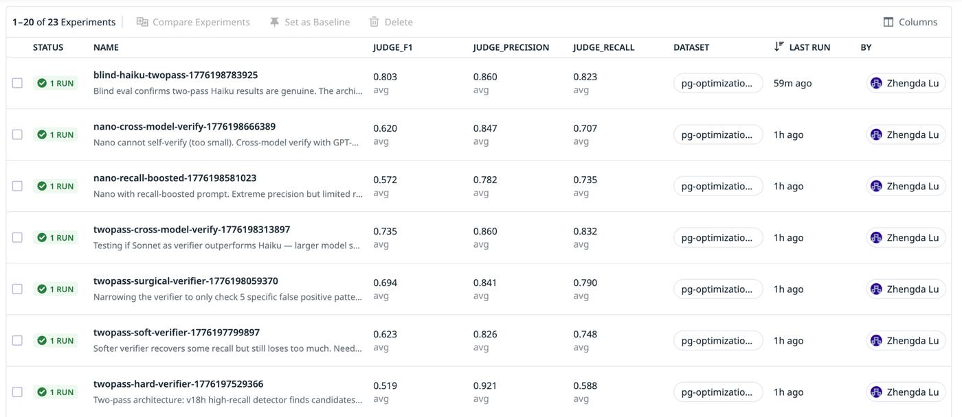
Once the dataset was in place, the team configured evaluators to measure the agent’s performance. These included precision, recall, and F1 scores. This way, they could compare the precision-recall tradeoff achieved in each agent iteration with a single heuristic marker (F1), as well as compare precision and recall scores across experiments. The following screenshot shows how these evaluators are displayed for each experiment run in LLM Observability Experiments.
Karpathy’s autoresearch is a setup where you give an AI agent a small but real LLM training codebase and let it experiment autonomously overnight. The agent modifies train.py, trains for five minutes, checks if the result improved, keeps it or discards it, and repeats. You wake up in the morning to a log of experiments and a better agent.
The design is deliberately simple:
One GPU
One file the agent edits (train.py)
One metric (validation bits per byte)
One file the human edits (program.md, the instructions that define the research direction).
The key idea is that humans are not designing individual experiments. The team sets parameters for the research by writing program.md, and the agent does the rest: proposing changes, running experiments, evaluating results, and deciding what to try next. The agent runs about 12 experiments per hour—roughly 100 overnight.
While autoresearch is designed to optimize model training, the DBM team wanted to apply the same methodology to AI agent development, where the “weights” being tuned are prompts, skills, and tools rather than neural network parameters. The DBM team adapted Karpathy’s tool to iterate the SQL optimization agent; 23 experiments produced 17 kept improvements.
In this case, the configured evaluators form the objective function that the autoresearch agent loop optimizes against. First, the team set a concrete target for this function: P>=0.85, R>=0.85 on a small model. Then, they set a fixed time budget of 15 minutes for each experiment run. Finally, they defined the intended agent behavior in a HANDOFF.md document. This document defines the current state, the error analysis, and the next hypotheses. A coding agent running in the autoresearch environment reads the handoff, designs experiments, runs them via LLM Observability Experiments, analyzes per-case failures, and writes the updated handoff for the next session.
Experiment code for one of these autoresearch runs is shown in the following snippet:
def optimization_task(input_data, config=None):
"""Your agent, wrapped as an experiment task."""
return run_optimization(
sql=input_data["sql"],
telemetry=input_data["telemetry"],
model=config.get("model", "anthropic/claude-haiku-4-5"),
)
experiment = LLMObs.experiment(
name="haiku-self-verify",
task=optimization_task,
dataset=dataset,
evaluators=[judge_precision, judge_recall, judge_f1],
config={
"model": "claude-haiku-4-5",
"prompt_version": "v20h",
"phase": "distillation",
"goal": "Add self-verification step to boost precision",
"expectation": "+2pp P from double-checking before output"
},
description="Self-verification: model reviews each suggestion against evidence before including it.",
)
result = experiment.run(jobs=10)
Each experiment is tagged with the hypothesis (goal), the prediction (expectation), and the research phase. LLM Observability Experiments records all of this as structured metadata alongside the per-case results and agent traces. When the automated driver analyzes failures in the next iteration, this metadata is what it reads to decide what to try next.
The experiment ran in two phases of eight experiments each: first, optimizing the agent’s system prompt, tool descriptions, and worked examples on a large model, and then finding the best way to compress to a smaller model while retaining the desired evaluation targets. The first two phases produced a result just beneath the target precision score of 0.85. A third phase ran seven more experiments to implement a two-pass solution that finally reached the team’s target. In this section, we’ll discuss how the agent was iterated through each of these phases.
In Phase 1, the autoresearch loop ran eight experiments on Claude Sonnet 4.6, starting with a zero-shot prompt (P=0.543, R=0.898) and iterating across three levers: the system prompt, the tool descriptions, and the worked examples.
The agent used seven tools that mirror production telemetry APIs: get_table_schema, get_explain_plans, get_query_metrics, get_idle_in_transaction_stats, and others. Early experiments focused on how the prompt instructs the agent to use these tools and interpret their output.
These runs produced three key turning points:
Structured output and evidence rules pushed precision from 0.54 to 0.83 across the first few experiments. Requiring the agent to cite tool evidence (explain plan costs, schema indexes) before suggesting optimizations eliminated most hallucinations.
Relaxing rules regressed. One experiment loosened missing-index co-occurrence rules, hoping to recover recall. Both precision and recall dipped.
Worked examples broke through. Adding three examples of what not to optimize (high-selectivity scans, subqueries with OFFSET, stale statistics) pushed precision to 0.878 while holding recall at 0.858.
After these iterations, blind evaluation on 50 more unseen cases confirmed no overfitting: P=0.870, R=0.830, as shown in the following screenshot:
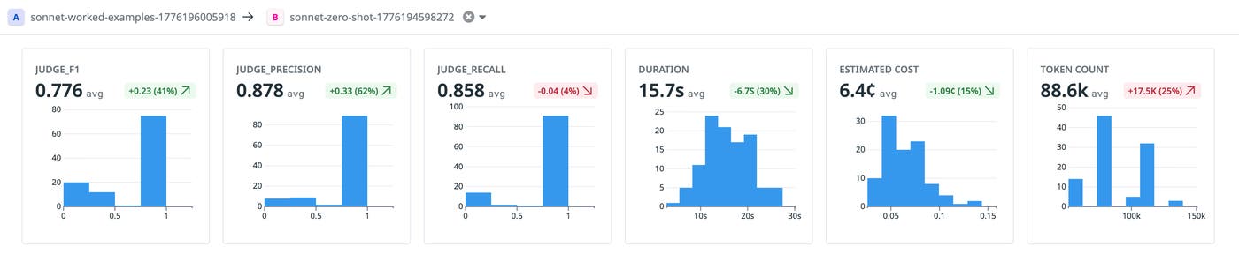
This view in LLM Observability Experiments lets you compare two experiments side by side. Here, we compare the initial zero-shot starting point against the final result of Phase 1. The precision gain is clear: The Phase 1 version’s precision was 61.6% higher.
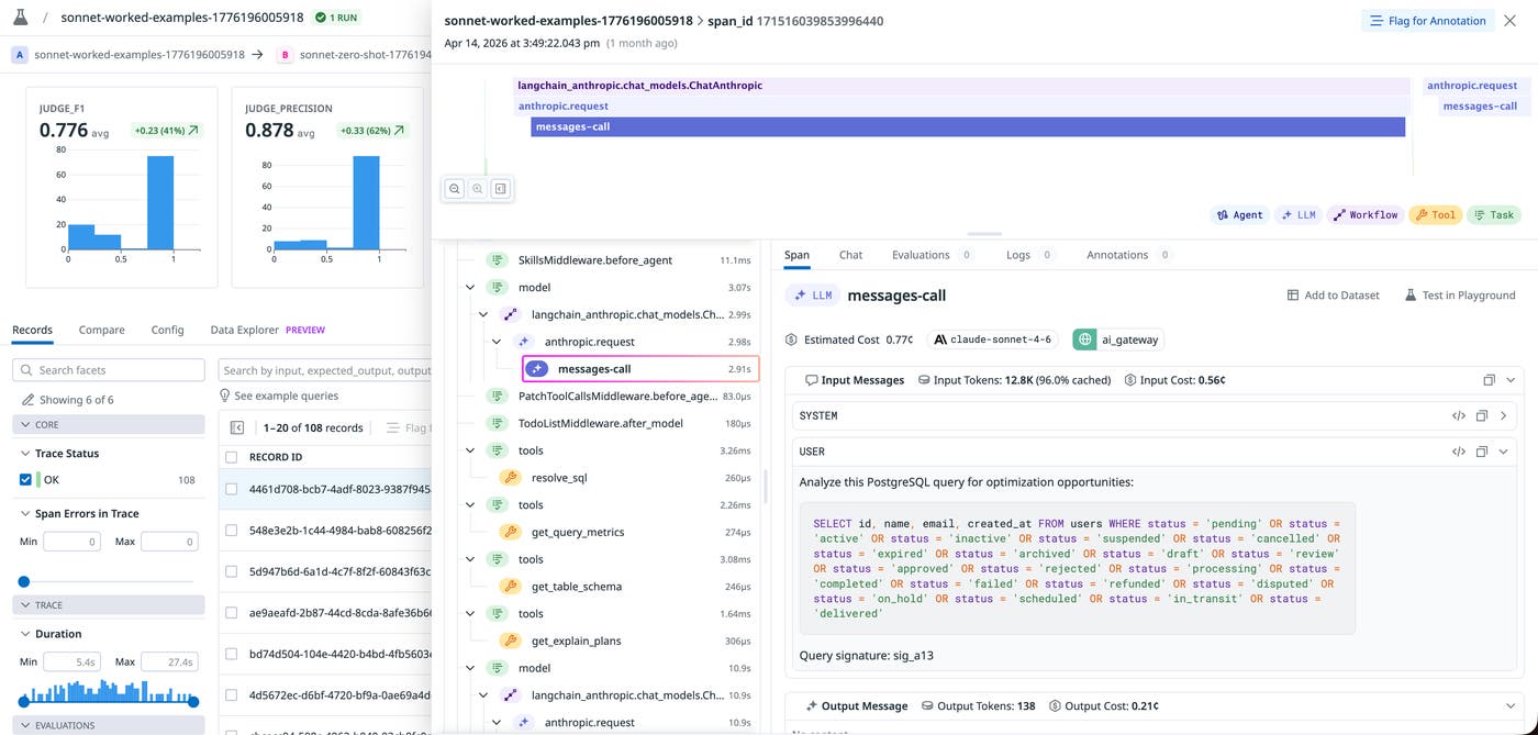
The team could also review full traces of this experiment run within LLM Observability’s trace visualization. In the following screenshot, we can see how the agent called resolve_sql, get_explain_plans, get_query_metrics, and get_table_schema before producing its recommendation.
Claude Sonnet 4.6 worked well for Phase 1, but at three times the cost of Haiku 4.5 ($3 input/$15 output per MTok versus $1 input/$5 output per MTok), it made sense to see if the quality gains could be compressed to the smaller model. The autoresearch driver explored two approaches for this.
First, it tried to directly transfer the Sonnet prompt to Haiku and find optimizations. Iterations that streamlined the prompt and added more worked examples failed to make up the response quality deficit introduced by running the original prompt on Haiku instead of Sonnet.
Applying a more rigorous, knowledge distillation–style approach broke through the challenge. The agent compared Sonnet and Haiku traces on the same cases in LLM Observability. In cases where Haiku got the wrong answer, the agent could directly compare with Sonnet for the same input and see exactly how it reasoned: which tools it called, what evidence it weighed, and how it arrived at the correct optimization type. The traces revealed that Haiku was confusing missing indexes with stale statistics and schema changes. The agent extracted four examples from Sonnet’s correct reasoning and added them to Haiku’s prompt. Both precision and recall improved.
The loop also experimented with on-demand skills: reusable instructions the agent can invoke for specific tasks like evidence gathering for missing index recommendations. Combining all hypotheses (distilled examples, skills, tool call hints) at once was unstable, but selective combinations worked better. The best single-pass Haiku version used distilled examples plus a self-verification step.
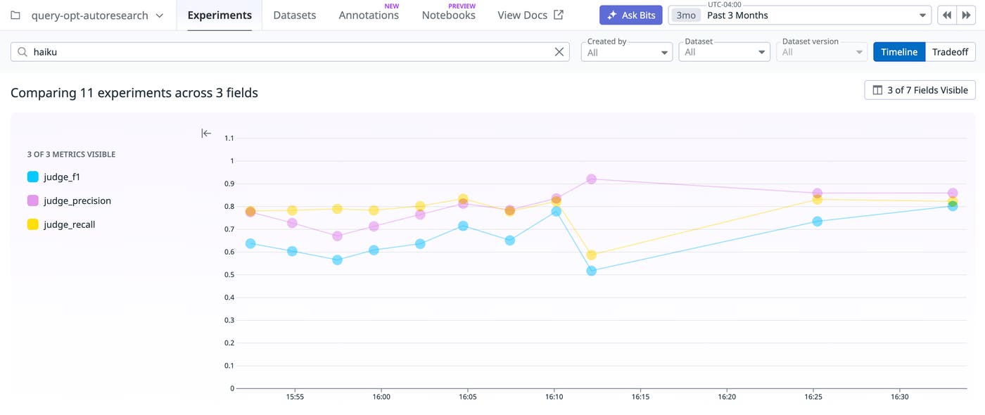
After another blind evaluation on 50 unseen cases, the agent confirmed that the new Haiku prompts generalize. Filtering by model name in LLM Observability surfaces just the Haiku experiments, making it easy to track progress within a single model family. The following screenshot shows the results of this test: P=0.837, R=0.823.
These results were strong, but just shy of the P=0.85 target the team had set. However, the autoresearch driver couldn’t find a way to improve them any further while sticking to a single Haiku call. The driver proposed splitting the problem into two passes: a high-recall detector followed by a surgical verifier.
The first iteration of the verifier was too aggressive and significantly reduced recall (P=0.921, R=0.588). The second was too soft to bring precision above the bar. The third struck the best balance by checking only five specific false-positive patterns identified through per-case error analysis.
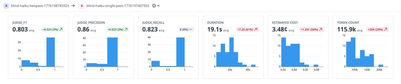
The autoresearch agent also tested cross-model verification (Sonnet as a verifier for Haiku) and distillation to GPT-5.4 nano. But the aforementioned Sonnet-only approach worked the best. A final blind evaluation check on 50 unseen cases produced P=0.860, R=0.823, F1=0.803, as shown in the following screenshot.
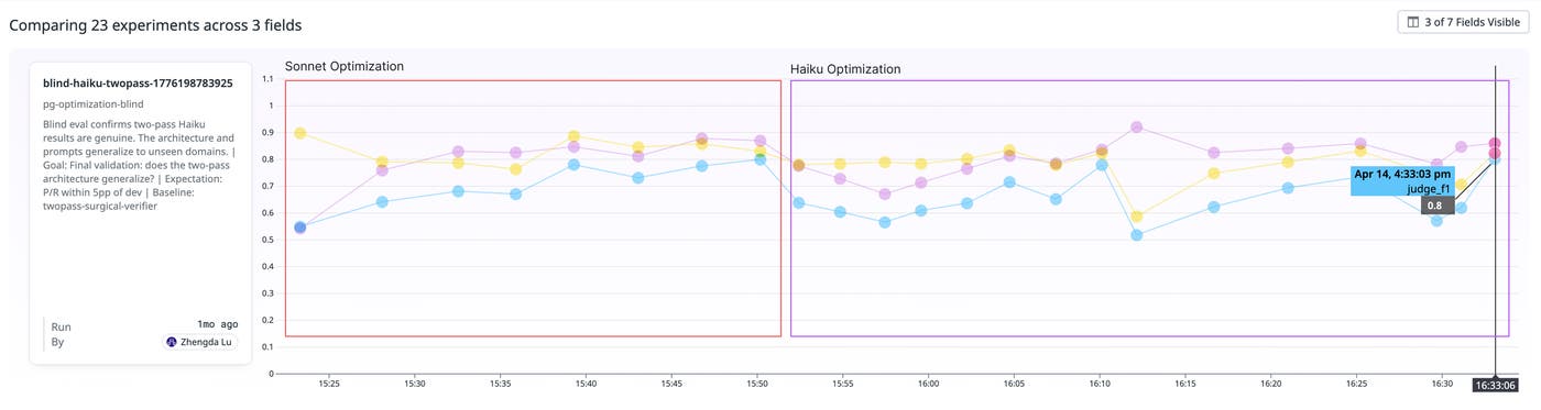
The following graph shows the full journey taken by the autoresearch agent. It performed 23 experiments across three phases. Each discarded experiment narrowed the search space and informed the next hypothesis. 17 improvements were kept, while 6 were discarded. F1 progressed from 0.550 (zero-shot) to 0.803 (two-pass Haiku).
At each step, the autoresearch reasoning and analysis output was saved to the corresponding experiment in LLM Observability Experiments as an audit log. This experiment infrastructure made it easy for the DBM team to track and analyze each step of this process, so they could find key learnings and understand what the autoresearch system had produced. LLM Observability Experiments enabled this by making every experiment a first-class object with:
Every experiment records its configuration (model, prompt version, variables changed), its hypothesis (goal and expectation tags), and its results (per-case precision, recall, and F1 from the LLM judge). There is no “I think we tried that,” because the experiment list shows exactly what was tried and what happened. It’s also easy to surface experiments with common attributes (model or prompt version, tool path, etc.) and compare their evaluator scores. This makes validating experiments’ performance gains much simpler and more reliable.
When an experiment regresses, you need to understand why at the case level. LLM Observability Experiments captures the full agent trace for every case: which tools were called, what the model reasoned about, and what it produced. We used this to discover that Haiku was recommending new indexes when the real problem was stale statistics, which directly informed the distillation examples.
Each experiment is tagged with phase, model family, and the variable that was changed (prompt, example, architecture). Filtering by haiku surfaces just the 11 Haiku experiments. Grouping by variable type reveals that architecture changes produced the biggest gains. These queries let you ask, “What have we tried on this model?” and get an answer in seconds.
Every experiment command is deterministic: the same dataset, the same model, the same prompt version. If a result looks surprising, you can rerun the experiment and compare. The loop ran blind evals after each phase specifically because the experiment infrastructure made it cheap to do so.
The autoresearch loop produces experiments at a pace that overwhelms manual tracking. At four to eight experiments per session, the research history becomes unmanageable within a week. By supporting this process with LLM Observability Experiments, the DBM team was able to make the system practical and sustainable.
This agentic experimentation methodology works for any AI agent, not just query optimization. The ingredients:
An evaluation dataset with real inputs, expected outputs, and metadata
A task function that wraps your agent
Evaluators that score output quality
The loop: hypothesize, experiment, measure, keep or discard
To learn more about running your own experiments, see our guide for building offline evaluations, and dive into the LLM Observability Experiments documentation. LLM Observability now has a free tier for your first 40,000 LLM spans. If you’re new to Datadog, sign up for a 14-day free trial.
此内容由惯性聚合(RSS阅读器)自动聚合整理,仅供阅读参考。 原文来自 — 版权归原作者所有。