There can be some practical constraints when it comes to deploying the AI models for retail environments. Retail environments can include store-level systems, edge devices, and budget conscious setup, especially for small to medium-sized retail companies. One such major use case is demand forecasting for inventory management or shelf optimization. It requires the deployed model to be small, fast, and accurate.

That is exactly what we will work on here. In this article, I will walk you through three compression techniques step by step. We will start by building a baseline LSTM. Then we will measure its size and accuracy, and then apply each compression method one at a time to see how it changes the model. At the end, we will bring everything together with a side-by-side comparison.

So, without any delay, let’s dive right in.

The Problem: Retail AI at the Edge

As everything is now moving to the edge, Retail is also moving towards store-level mobile apps, devices, and IOT sensors, which can run the models and predict the forecast locally rather than calling the cloud APIs every time.

A forecast model running on a store device or mobile app, like a shelf sensor or scanner, can face constraints such as limited memory, limited battery, and requires low network latency.

Even for cloud deployments, if the model size is smaller, it can lower the costs. Especially when you are running thousands of predictions daily across a huge product catalog. A model with size 4KB costs significantly less than a model with size 64KB

Not just cost, inference speed also affects the real-time decisions. Faster model prediction can benefit inventory optimization and restocking alerts.

Benchmarking Setup

For the experiment, I utilized the Kaggle Item Demand forecasting data set at the store level. The data is spread over 5 years of daily sales across 10 stores and 50 items. This public data set has a retail pattern with weekly seasonality, trends, and noise.

For this, I used sample data of 5 stores, 10 items, and created 50 separate time series. Each of the store item combinations generates its own sequences, which will result in a total of 72,000 training sample data. The model will predict the next day’s sales data based on the past 14 days’ sales history, which is a common setup for demand forecasting data.

The experiment was run 3 times and averaged for reliable results.

Step 1: Building the Baseline LSTM

Before compressing anything, we need a reference point. Our baseline is a standard LSTM with 64 hidden units trained on the dataset described above.

Baseline Code:

from tensorflow.keras.models import Sequential
from tensorflow.keras.layers import LSTM, Dense, Dropout
def build_lstm(units, seq_length):
    """Build LSTM with specified hidden units."""
    model = Sequential([
        LSTM(units, activation='tanh', input_shape=(seq_length, 1)),
        Dropout(0.2),
        Dense(1)
    ])
    model.compile(optimizer='adam', loss='mse')
    return model
# Baseline: 64 hidden units
baseline_model = build_lstm(64, seq_length=14) 

Baseline Performance:

This is our reference point. The LSTM-64 model is 66.25KB in size with a MAPE of 15.92%. Every compression technique below will be measured against these numbers.

Step 2: Compression Technique 1 — Architecture Sizing

In this approach, we reduce the model capacity by a few hidden units. Instead of a 64-unit LSTM, we train a 32/16-unit model from scratch and see how it performs. This is a simpler approach among the three.

Code:

# Using the same build_lstm function from baseline
# Compare: 64 units (66KB) vs 32 units vs 16 units
model_32 = build_lstm(32, seq_length=14)
model_16 = build_lstm(16, seq_length=14)

Results:

Analysis: The LSTM-16 model is 14.5x smaller than 64 bit model (4.57KB vs 66.25KB), while MAPE is increased only by 0.82%. For a lot of applications in retail, this difference is minute, whereas the LSTM 32 model offers a middle ground with 3.9x compression, having 0.3% accuracy loss.

Step 3: Compression Technique 2 — Magnitude Pruning

Pruning is to remove low-importance weights from model training. The core idea is that the contributions of many neural network connections are minimal and can be ignored or set to zero. After the pruning, the model is fine-tuned to recover the accuracy.

Code:

import numpy as np
from tensorflow.keras.optimizers import Adam
def apply_magnitude_pruning(model, target_sparsity=0.5):
    """Apply per-layer magnitude pruning, skip biases"""
    masks = []
    for layer in model.layers:
        weights = layer.get_weights()
        layer_masks = []
        new_weights = []
        for w in weights:
            if w.ndim == 1:  # Bias - don't prune
                layer_masks.append(None)
                new_weights.append(w)
            else:  # Kernel - prune per-layer
                threshold = np.percentile(np.abs(w), target_sparsity * 100)
                mask = (np.abs(w) >= threshold).astype(np.float32)
                layer_masks.append(mask)
                new_weights.append(w * mask)
        masks.append(layer_masks)
        layer.set_weights(new_weights)
    return masks
# After pruning, fine-tune with lower learning rate
model.compile(optimizer=Adam(learning_rate=0.0001), loss='mse')
model.fit(X_train, y_train, epochs=50, callbacks=[maintain_sparsity])

Results:

Analysis: With Magnitude Pruning at 50% sparsity, the model size has dropped to 8.56KB with only 0.28% accuracy loss compared to the baseline. Even with 70% Pruning, MAPE was under 17%.

The important finding to make pruning work on LSTMs was using thresholds at every layer instead of a global threshold, skipping bias weights (using only kernel weights), and also using a lower learning rate during fine-tuning. Without these, LSTM performance can degrade significantly due to the interdependency of recurrent weights.

Step 4: Compression Technique 3 — INT8 Quantization

Quantization deals with the conversion of 32-bit floating point weights to 8-bit integers post-training which will reduce the model size by 4 times without losing much of accuracy.

Code:

def simulate_int8_quantization(model):
    """Simulate INT8 quantization on model weights."""
    for layer in model.layers:
        weights = layer.get_weights()
        quantized = []
        for w in weights:
            w_min, w_max = w.min(), w.max()
            if w_max - w_min > 1e-10:
                # Quantize to INT8 range [0, 255]
                scale = (w_max - w_min) / 255.0
                zero_point = np.round(-w_min / scale)
                w_int8 = np.round(w / scale + zero_point).clip(0, 255)
                # Dequantize
                w_quant = (w_int8 - zero_point) * scale
            else:
                w_quant = w
            quantized.append(w_quant.astype(np.float32))
        layer.set_weights(quantized)

For production deployment, it’s recommended to use TensorFlow Lite’s built-in quantization:

import tensorflow as tf
converter = tf.lite.TFLiteConverter.from_keras_model(model)
converter.optimizations = [tf.lite.Optimize.DEFAULT]
tflite_model = converter.convert()

Results:

Analysis: INT8 quantization has reduced the model size to 4.28KB from 66.25KB(15.5x compression) with 0.29% increase in accuracy. This is the smallest model with accuracy comparable to the unpruned LSTM 32 model. Specially for deployments, INT8 inference is supported, and it is the best among 3 techniques.

Bringing It All Together: Side-by-Side Comparison

Here’s how each technique compares against the LSTM-64 baseline:

The full benchmark results across all techniques:

Each one of the above techniques comes with its own tradeoffs. Architecture sizing can reduce the model size, but it needs retraining of the model. Pruning will preserve the architecture but filters the connections. Quantization can be fast but requires compatible inference runtimes.

Choosing the Right Technique

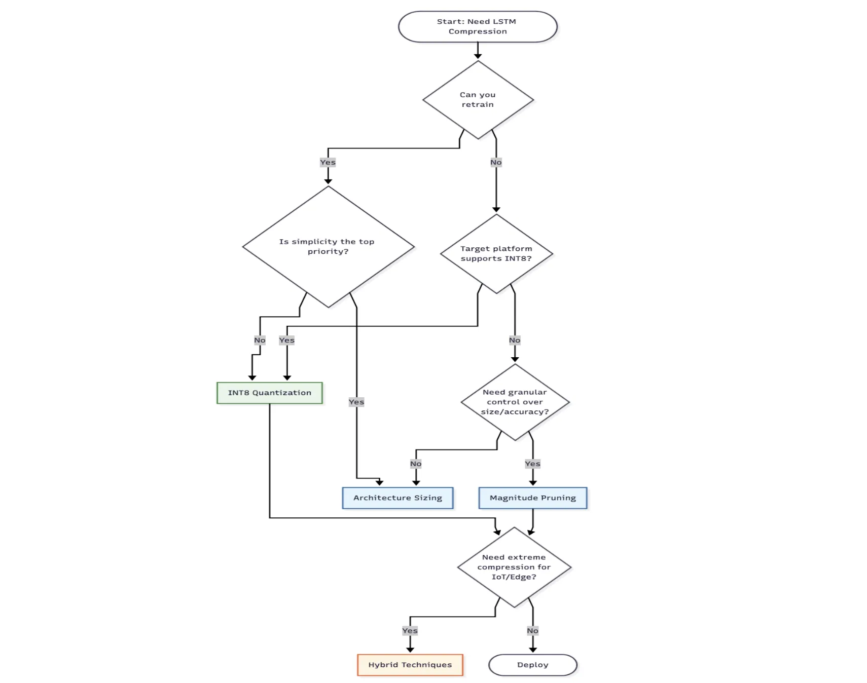
Choose Architecture Sizing when:

• You’re starting from scratch and can train
• Simplicity matters more than maximum compression

Pick Pruning when:

• You already have a trained model and are looking for model compression
• You need granular-level control over the accuracy-size tradeoff

Go for Quantization when:

• You need maximum compression with minimal accuracy loss
• Your target deployment platform has INT8 optimization (Ex, mobile, edge devices)
• You want a quick solution without retraining from the beginning.

Choose hybrid techniques when:

• Heavy compression is required (edge deployment, IoT)
• You can invest time in iterating on the compression pipeline

Points to Remember for Retail Deployment

Model compression is just one part of the puzzle. There are other factors to consider for retail systems, as given below.

1. A Larger model is always better than a smaller model which is stale. Build retraining into your pipeline as retail patterns change with seasons, trends, promotions, etc.
2. Benchmarks from a local machine cannot be matched with a production environment device. Especially, the quantized models can behave differently on different platforms.
3. Monitoring is a key element in production, as compression can cause subtle accuracy degradation. All necessary alerts and paging must be in place.
4. Always consider the entire system cost as a 4KB model that needs a specialized sparse inference runtime might cost more than deploying a regular 17KB model, which runs everywhere.

Conclusion

To conclude, all three compression techniques can deliver significant size reductions while maintaining proper accuracy.

Architecture sizing is the simplest among 3. An LSTM-16 delivers 14.5x compression with less than 1% accuracy loss.

Pruning offers more control. With proper execution (per-layer thresholds, skip biases, low learning rate fine-tuning), 70% pruning achieves 12.9x compression.

INT8 quantization achieves the best tradeoff with 15.5x compression with only 0.29% increase in accuracy.

Choosing the best technique will depend on your limitations and constraints. If a simple solution is needed, then start with architecture sizing. If needed, a maximum level of compression with minimal accuracy loss, go with quantization. Choose pruning mainly when you need a fine-grained control over the compression accuracy tradeoff.

For edge deployments that help the in-store devices, tablets, shelf sensors, or scanners, the model size (4KB vs 66KB) can determine if your AI runs locally on the device or require a continuous cloud connectivity.