OpenCV Recipes：图像的几何变换

Wang's Blog

【Atlas 移植训练营极市×昇腾】 Atlas 移植初体验使用vcpkg和CMake在vs code与clion中构建Qt应用生成对抗网络（GANs）机器学习中的一阶与随机优化方法：机器学习模型 Savitzky-Golay 滤波平滑与n阶导数系数的推导经典CS问题Python实现：搜索问题图像挖掘中Canny和Sobel边缘检测算法的性能分析经典CS问题Python实现：简单问题 Design Patterns Used in Qt and OpenCV Jaya 优化算法及其变体萤火虫算法遗传算法模拟退火随机行走与最优化自然启发式算法算法分析机器学习之 TensorFlow 基础数值 Python: 常微分方程数值 Python: 求解方程差分进化算法

Wang Xin · 2018-06-25 · via Wang's Blog

In this post, we are going to learn how to apply cool geometric effects to images.

读取、显示与保存图像

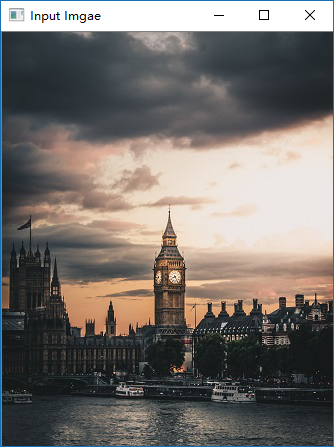
确保当前目录下有一个名为 input.jpg 的文件，现在，让我们创建一个名为 load_and_show.py 的文件，输入以下内容到文件中。

import cv2

img = cv2.imread('input.jpg')
cv2.imshow('Input Imgae', img)
cv2.waitKey()

运行脚本，会显示图像。

引用的图片来源信息：

Photo by Luke Stackpoole on Unsplash
Luke Stackpoole
@withluke
Big Ben, London, United Kingdom
IG: @WithLuke // info@withluke.com

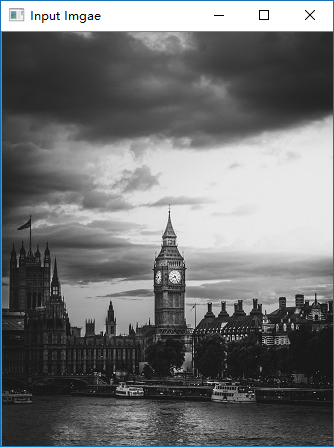
让我们以灰度模式显示图像

import cv2

img = cv2.imread('input.jpg', cv2.IMREAD_GRAYSCALE)
cv2.imshow('Input Imgae', img)
cv2.waitKey()

我们就得到了灰度图

保存得到的灰度图

import cv2

img = cv2.imread('input.jpg', cv2.IMREAD_GRAYSCALE)
cv2.imshow('Input Imgae', img)
cv2.imwrite('output.jpg', img)
cv2.waitKey()

将原始图片格式变为 PNG 格式

import cv2

img = cv2.imread('input.jpg', cv2.IMREAD_GRAYSCALE)
cv2.imshow('Input Imgae', img)
cv2.imwrite('output.png', img, [cv2.IMWRITE_PNG_COMPRESSION])
cv2.waitKey()

这里使用了 ImwriteFlag 中的 IMWRITE_PNG_COMPRESSION，更多内容请参考 ImwriteFlags

图像色彩空间

有很多有用的色彩空间，其中流行的有 RGB、YUV 和 HSV 等。可以通过以下 Python 脚本列出 OpenCV 所有可能色彩空间转换选项。

1
2
3

import cv2

print([x for x in dir(cv2) if x.startswith('COLOR_')])

可以将任何色彩空间转换成另一种色彩空间，如将彩色图像转换为灰度图像

import cv2

img = cv2.imread('input.jpg', cv2.IMREAD_COLOR)
gray_img = cv2.cvtColor(img, cv2.COLOR_RGB2GRAY)
cv2.imshow('Input Imgae', gray_img)
cv2.waitKey()

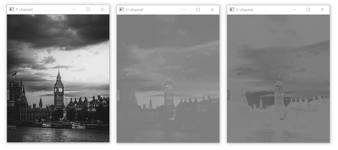
可以通过如下操作分离图像通道

import cv2

img = cv2.imread('input.jpg', cv2.IMREAD_COLOR)
yuv_img = cv2.cvtColor(img, cv2.COLOR_RGB2YUV)


cv2.imshow('Y channel', yuv_img[:, :, 0])
cv2.imshow('U channel', yuv_img[:, :, 1])
cv2.imshow('V channel', yuv_img[:, :, 2])







cv2.waitKey()

第一种分离方法使用的是 NumPy 数组的特性。我们得到下面三种通道的图像

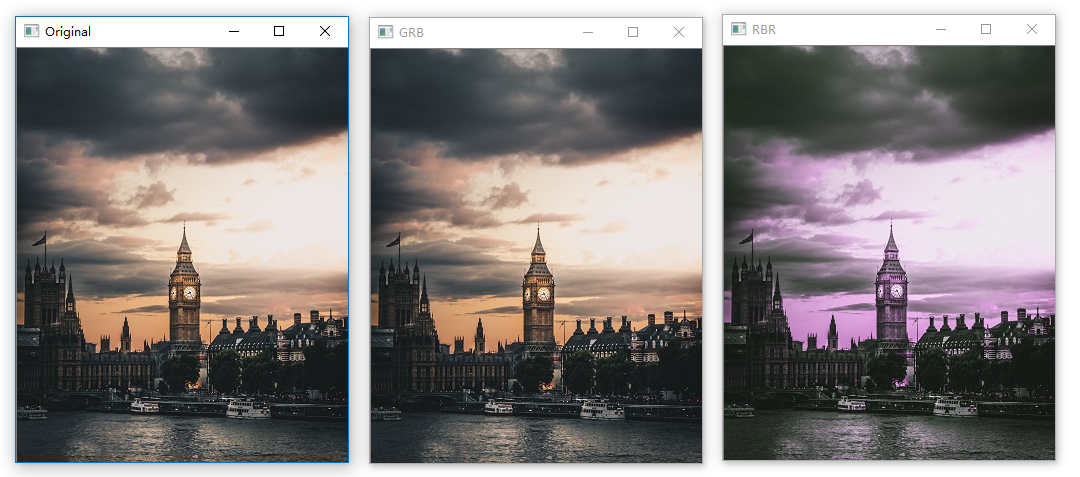
让我们看看不同通道组合在一起的效果

import cv2

img = cv2.imread('input.jpg', cv2.IMREAD_COLOR)

g, b, r = cv2.split(img)
gbr_img = cv2.merge((g, b, r))
rbr_img = cv2.merge((r, b, r))

cv2.imshow("Original", img)
cv2.imshow("GRB", gbr_img)
cv2.imshow("RBR", rbr_img)

cv2.waitKey()

图像变换

现在，让我们来平移图像

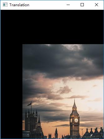
import cv2
import numpy as np

img = cv2.imread('input.jpg')

num_rows, num_cols = img.shape[:2]
translation_matrix = np.float32([[1, 0, 70], [0, 1, 110]])
img_translation = cv2.warpAffine(img, 
    translation_matrix, (num_cols, num_rows))

cv2.imshow('Translation', img_translation)
cv2.waitKey()

平移基本上意味着通过增加/减少 x 和 y 坐标来移动图像。为此，我们需要创建一个变换矩阵，如下所示：

$$
T =
\begin{bmatrix}
1 & 0 & t_x \
0 & 1 & t_y
\end{bmatrix}
$$

这里， $t_x$ 和 $t_y$ 值是 x 和 y 转换值；也就是说，图像将向右移动 x 个单位，向下移动 y 个单位。一旦我们创建了这样一个矩阵，我们就可以使用函数 warpAffine 将之应用到图像中。warpAffine 中的第三个参数用于指生成的图像的行数和列数。该函数还可传定义插值方法组合的 InterpolationFlags，具体请参考 InterpolationFlags。

可以发现上面的图像被裁切，为防止被裁切我们可以这样：

1	img_translation = cv2.warpAffine(img, translation_matrix, (num_cols+70, num_rows+110))

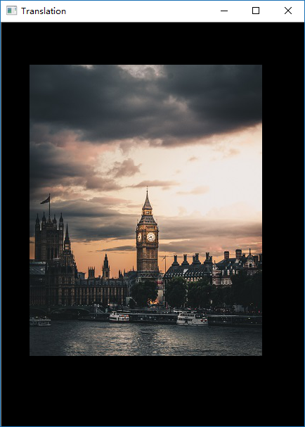
将图像移动到大框的中间，可以这样：

import cv2
import numpy as np

img = cv2.imread('input.jpg')

num_rows, num_cols = img.shape[:2]
translation_matrix = np.float32([[1, 0, 70], [0, 1, 110]])
img_translation = cv2.warpAffine(img, 
    translation_matrix, (num_cols+70, num_rows+110))
translation_matrix = np.float32([[1, 0, -30], [0, 1, -50]])
img_translation = cv2.warpAffine(img_translation, 
    translation_matrix, (num_cols+70+30, num_rows+110+50))

cv2.imshow('Translation', img_translation)
cv2.waitKey()

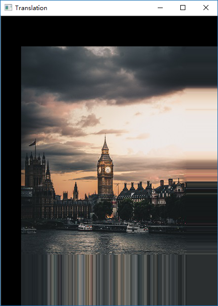
该函数还有 borderMode 和 borderValue 参数，允许通过像素外推法填充平移的空白边框。

import cv2
import numpy as np

img = cv2.imread('input.jpg')

num_rows, num_cols = img.shape[:2]
translation_matrix = np.float32([[1, 0, 70], [0, 1, 110]])
img_translation = cv2.warpAffine(img, 
    translation_matrix, (num_cols+70, num_rows+110))
translation_matrix = np.float32([[1, 0, -30], [0, 1, -50]])
img_translation = cv2.warpAffine(img_translation, 
    translation_matrix, (num_cols+70+30, num_rows+110+50), 
    cv2.INTER_LINEAR, cv2.BORDER_WRAP, 1)

cv2.imshow('Translation', img_translation)
cv2.waitKey()

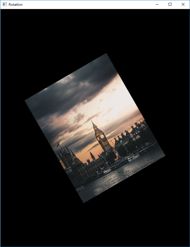
可以通过以下操作将给定图像旋转特定角度。

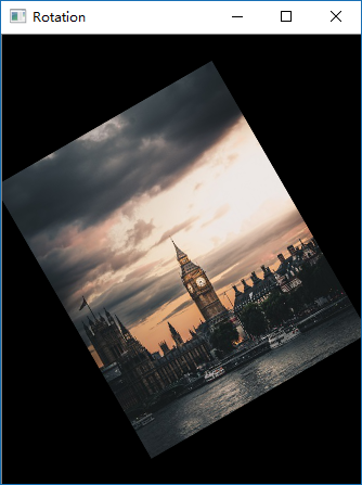
import cv2
import numpy as np

img = cv2.imread('input.jpg')

num_rows, num_cols = img.shape[:2]
rotation_matrix = cv2.getRotationMatrix2D((num_cols/2, num_rows/2), 30, 0.7)
img_rotation = cv2.warpAffine(img, rotation_matrix, (num_cols, num_rows))

cv2.imshow('Rotation', img_rotation)
cv2.waitKey()

使用 getRotationMatrix2D，我们可以指定图像围绕旋转的中心点作为第一个参数，然后指定旋转角度（以度为单位），最后指定图像的缩放因子。

旋转也是一种变换形式，我们可以用下面的变换矩阵来实现：

$$
R =
\begin{bmatrix}
\cos \theta & -\sin \theta \
\sin \theta & \cos \theta
\end{bmatrix}
$$

这里 θ 是逆时针方向的旋转角度。OpenCV 通过 getRotationMatrix2D 函数提供了对创建此矩阵的更好控制。一旦我们有了变换矩阵，我们就可以用 warpAffine 函数将该矩阵应用于任何图像。

从上图中可以看出，图像内容超出界限，被轻微裁剪。为了防止这种情况，我们需要在输出图像中提供足够的空间。让我们继续使用前面讨论的变换功能来执行此操作：

import cv2
import numpy as np

img = cv2.imread('input.jpg')

num_rows, num_cols = img.shape[:2]

translation_matrix = np.float32([[1, 0, int(0.5*num_cols)], 
    [0, 1, int(0.5*num_rows)]])
rotation_matrix = cv2.getRotationMatrix2D((num_cols, num_rows), 30, 1)

img_translation = cv2.warpAffine(img, translation_matrix, 
    (2*num_cols, 2*num_rows))
img_rotation = cv2.warpAffine(img_translation, rotation_matrix, 
    (num_cols*2, num_rows*2))

cv2.imshow('Rotation', img_rotation)
cv2.waitKey()

图像缩放

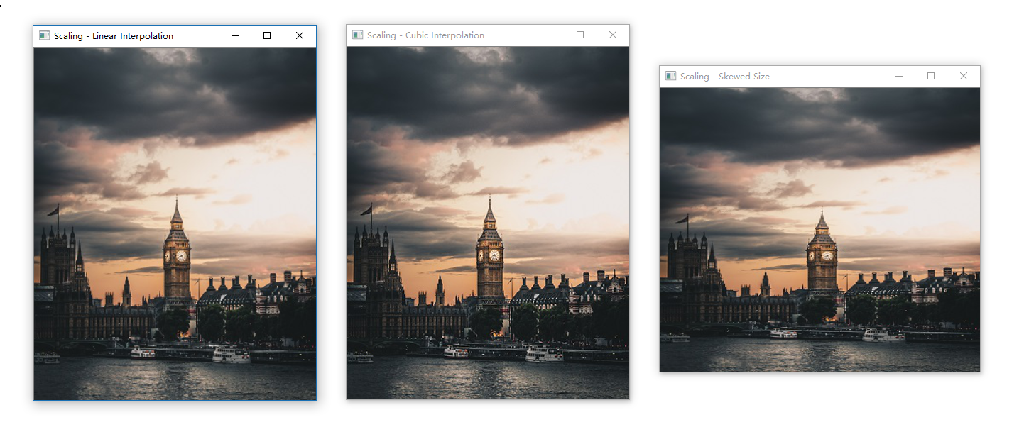
现在，让我们将图片缩放到特定大小。

import cv2

img = cv2.imread('input.jpg')

img_scaled = cv2.resize(img, None, fx=1.2, fy=1.2, 
    interpolation=cv2.INTER_LINEAR)
cv2.imshow('Scaling - Linear Interpolation', img_scaled)

img_scaled = cv2.resize(img, None, fx=1.2, fy=1.2, 
    interpolation=cv2.INTER_CUBIC)
cv2.imshow('Scaling - Cubic Interpolation', img_scaled)

img_scaled = cv2.resize(img, (450, 400), interpolation=cv2.INTER_AREA)
cv2.imshow('Scaling - Skewed Size', img_scaled)

cv2.waitKey()

仿射变换

下面，我们将讨论二维图像的各种广义几何变换。在讨论仿射变换（affine transformations）之前，让我们先了解欧几里得变换是什么。欧几里得变换是一种保留长度和角度度量的几何变换。如果我们对几何形状应用欧几里得变换，则该形状将保持不变。它可能会发生旋转、移位等，但基本结构不会改变。所以从技术上讲，线将保持直线，平面将保持平面，正方形将保持正方形，圆将保持圆。

现在，回到仿射变换，我们可以说它们是欧几里得变换的推广。在仿射变换的范围内，线将保持直线，但正方形可能变成矩形或平行四边形。基本上，仿射变换不保留长度和角度。

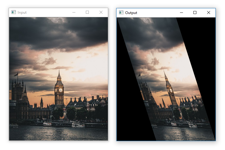
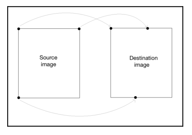
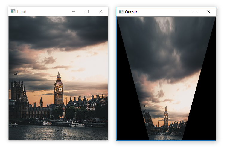
为了建立一般的仿射变换矩阵，需要定义控制点。一旦我们有了这些控制点，我们还需要确定将它们映射到哪里。在这种特殊情况下，我们需要的只是源图像中的三点，以及输出图像中的三点。让我们看看如何将图像转换成类平行四边形图像：

import cv2
import numpy as np

img = cv2.imread('input.jpg')

rows, cols = img.shape[:2]
src_points = np.float32([[0, 0], [cols - 1, 0], [0, rows - 1]])
dst_points = np.float32([[0, 0], [int(0.6*(cols - 1)), 0], 
    [int(0.4*(cols - 1)), rows - 1]])
affine_matrix = cv2.getAffineTransform(src_points, dst_points)
img_output = cv2.warpAffine(img, affine_matrix, (cols, rows))

cv2.imshow('Input', img)
cv2.imshow('Output', img_output)
cv2.waitKey()

上面代码的映射关系如下图所示。

射影变换

仿射变换有一些限制，而射影变换则给了我们更多的自由。为了理解射影变换，我们需要理解射影几何是如何工作的。例如，如果你正站在一张纸上画了一个正方形的前面，它看起来就像一个正方形。
现在，如果你开始倾斜那张纸，正方形会越来越像梯形。射影变换允许我们用一种很好的数学方法捕捉这种动态。这些变换既不保留大小也不保留角度，但保留了入射角和交叉比（cross-ratio）。

现在我们已经知道射影变换是什么了，让我们看看是否可以在这里提取更多的信息。可以说，给定平面上的任意两幅图像都是由单应性相关的。只要它们在同一平面上，我们就可以把任何东西转换成任何东西。这具有许多实际应用，例如增强现实、图像校正、图像配准或计算两幅图像之间相机的运动。

一旦从估计的单应矩阵中提取了相机旋转和平移，该信息就可以用于导航，或者将 3D 对象的模型插入图像或视频中。这样一来，它们就以正确的视角呈现，看起来就像是原始场景的一部分。

import cv2
import numpy as np

img = cv2.imread('input.jpg')
rows, cols = img.shape[:2]

src_points = np.float32([[0, 0], [cols - 1, 0], 
    [0, rows - 1], [cols - 1, rows - 1]])
dst_points = np. float32([[0, 0], [cols - 1, 0], 
    [int(0.33*cols), rows - 1], [int(0.66*cols), rows - 1]])

projective_matrix = cv2.getPerspectiveTransform(src_points, dst_points)
img_output = cv2.warpPerspective(img, projective_matrix, (cols, rows))

cv2.imshow('Input', img)
cv2.imshow('Output', img_output)

cv2.waitKey()

我们可以在源图像中选择四个控制点，并将它们映射到目标图像。平行线在转换后不会保持平行线。我们使用 getProjectiveTransform 函数来得到转换矩阵。

图像扭曲

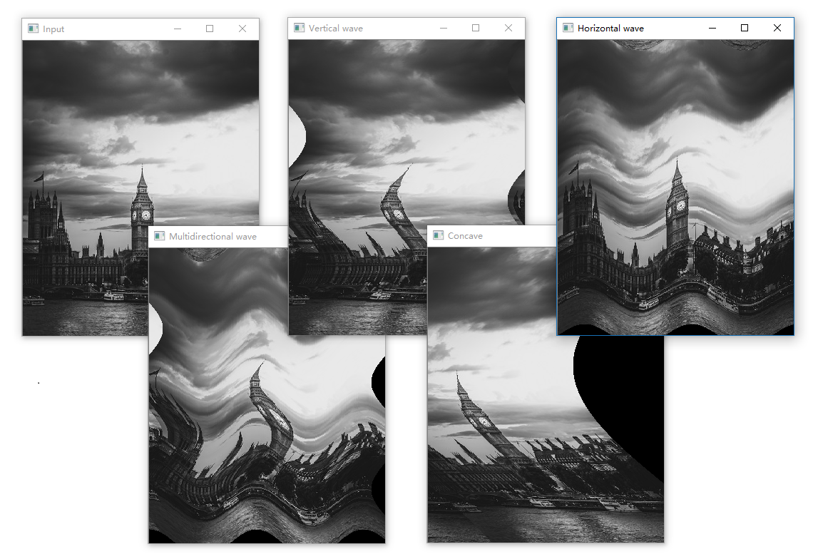
现在，让我们实现一些有趣的效果。

import cv2
import numpy as np
import math


img = cv2.imread('input.jpg', cv2.IMREAD_GRAYSCALE)

rows, cols = img.shape


img_output = np.zeros(img.shape, dtype=img.dtype)

for i in range(rows):
    for j in range(cols):
        offset_x = int(25.0*math.sin(2*3.14*i / 180))
        offset_y = 0
        if j+offset_x < rows:
            img_output[i,j] = img[i,(j+offset_x)%cols]
        else:
            img_output[i,j] = 0

cv2.imshow('Input', img)
cv2.imshow('Vertical wave', img_output)


img_output = np.zeros(img.shape, dtype=img.dtype)

for i in range(rows):
    for j in range(cols):
        offset_x = 0
        offset_y = int(16.0*math.sin(2*3.14*j / 150))
        if i+offset_y < rows:
            img_output[i,j] = img[(i+offset_y)%rows,j]
        else:
            img_output[i,j] = 0

cv2.imshow('Horizontal wave', img_output)


img_output = np.zeros(img.shape, dtype=img.dtype)

for i in range(rows):
    for j in range(cols):
        offset_x = int(20.0*math.sin(2*3.14*i / 150))
        offset_y = int(20.0*math.cos(2*3.14*j / 150))
        if i+offset_y < rows and j+offset_x < cols:
            img_output[i,j] = img[(i+offset_y)%rows,(j+offset_x)%cols]
        else:
            img_output[i,j] = 0

cv2.imshow('Multidirectional wave', img_output)


img_output = np.zeros(img.shape, dtype=img.dtype)

for i in range(rows):
    for j in range(cols):
        offset_x = int(128.0 * math.sin(2 * 3.14 * i / (2*cols)))
        offset_y = 0
        if j+offset_x < cols:
            img_output[i,j] = img[i,(j+offset_x)%cols]
        else:
            img_output[i,j] = 0
            
cv2.imshow('Concave', img_output)
cv2.waitKey()

此内容由惯性聚合(RSS阅读器)自动聚合整理，仅供阅读参考。原文来自 — 版权归原作者所有。

推荐订阅源

Wang's Blog

读取、显示与保存图像

图像色彩空间

图像变换

图像缩放

仿射变换

射影变换

图像扭曲