




惯性聚合 高效追踪和阅读你感兴趣的博客、新闻、科技资讯
阅读原文 在惯性聚合中打开

推荐订阅源

Jina AI
Jina AI
宝玉的分享
宝玉的分享
Last Week in AI
Last Week in AI
Help Net Security
Help Net Security
让小产品的独立变现更简单 - ezindie.com
人人都是产品经理
人人都是产品经理
奇客Solidot–传递最新科技情报
奇客Solidot–传递最新科技情报
GbyAI
GbyAI
博客园_首页
freeCodeCamp Programming Tutorials: Python, JavaScript, Git & More
MongoDB | Blog
MongoDB | Blog
Cyber Security Advisories - MS-ISAC
L
LINUX DO - 最新话题
PCI Perspectives
PCI Perspectives
博客园 - 三生石上(FineUI控件)
V2EX - 技术
V2EX - 技术
Spread Privacy
Spread Privacy
T
Tor Project blog
量子位
阮一峰的网络日志
阮一峰的网络日志
S
SegmentFault 最新的问题
小众软件
小众软件
博客园 - 叶小钗
Threat Intelligence Blog | Flashpoint
Blog — PlanetScale
Blog — PlanetScale
H
Help Net Security
Y
Y Combinator Blog
N
News | PayPal Newsroom
K
KPMG report finds enterprise disconnect between AI and its ROI | CIO
T
Tenable Blog
Scott Helme
Scott Helme
G
GRAHAM CLULEY
大猫的无限游戏
大猫的无限游戏
aimingoo的专栏
aimingoo的专栏
IT之家
IT之家
Schneier on Security
F
Fortinet All Blogs
Martin Fowler
Martin Fowler
T
Threat Research - Cisco Blogs
博客园 - 司徒正美
Application and Cybersecurity Blog
钛媒体:引领未来商业与生活新知
钛媒体:引领未来商业与生活新知
Attack and Defense Labs
Exploit-DB.com RSS Feed
The Last Watchdog
The Last Watchdog
L
LangChain Blog
C
Check Point Blog
Google Online Security Blog
V
Visual Studio Blog
Latest news
Latest news

VictoriaMetrics: Simple & Reliable Monitoring for Everyone on VictoriaMetrics

Operator now has Long-Term Support (LTS) version Multi-tiered Observability: A Practical Way to Handle Diverse Workloads VictoriaMetrics April 2026 Ecosystem Updates Not All Telemetry Requires Premium Pricing VictoriaMetrics at KubeCon Amsterdam: Community Highlights What's new in VictoriaMetrics Anomaly Detection (Q1 2026) What's New in VictoriaMetrics Cloud Q1 2026? Logs, MCP Server, Better Alerting, and... a Secret Project VictoriaMetrics at KubeCon: Optimizing Tail Sampling in OpenTelemetry with Retroactive Sampling VictoriaMetrics March 2026 Ecosystem Updates Observability Lessons From OpenAI Benchmarking Kubernetes Log Collectors: vlagent, Vector, Fluent Bit, OpenTelemetry Collector, and more VictoriaMetrics February 2026 Ecosystem Updates VictoriaMetrics at FOSDEM, Cloud Native Days France, and CfgMgmtCamp Ghent VictoriaLogs in VictoriaMetrics Cloud: Fast, Cost-Effective Log Management is Here What’s new in VictoriaMetrics Anomaly Detection (2025) VictoriaMetrics January 2026 Ecosystem Updates VictoriaLogs Basics: What You Need to Know, with Examples & Visuals What's New in VictoriaMetrics Cloud Q4 2025? New tiers, more deployment options, IaC and alerting rules. Vibe coding tools observability with VictoriaMetrics Stack and OpenTelemetry How a US Software Provider Improved Traffic Alerting with VictoriaMetrics Anomaly Detection VictoriaMetrics 2025 Developer Experience: A Year in Review Spotify’s performance & control across large monitoring environments with VictoriaMetrics VictoriaMetrics Achieves Red Hat OpenShift Operator Certification Our latest updates across the VictoriaMetrics Observability ecosystem New Capacity Tiers in VictoriaMetrics Cloud Announcing 1B+ Downloads & Product Development With Logs, Traces, Metrics AI Agents Observability with OpenTelemetry and the VictoriaMetrics Stack Discarding gRPC-Go: The Story Behind OTLP/gRPC Support in VictoriaTraces What's New in VictoriaMetrics Cloud Q3 2025? From new region in Asia to proactive alerts How DreamHost Slashed Memory Usage by 80% and Scaled to 76 Million Time Series Upcoming Conferences & Meetups: Where to Meet Our Team VictoriaMetrics Long-Term Support (LTS): H2 2025 Update Creating a Sustainable Open Source Business Model - Introduction Full-Stack Observability with VictoriaMetrics in the OTel Demo Alerting Best Practices vmanomaly Deep Dive: Smarter Alerting with AI (Tech Talk Companion) VictoriaLogs Practical Ingestion Guide for Message, Time and Streams Monotonic and Wall Clock Time in the Go time package Hello Singapore! VictoriaMetrics Cloud Expands to Asia Pacific MCP Server Integration & Much More: What's New in VictoriaMetrics Cloud Q2 2025 FIPS 140-3 Compatible Builds for VictoriaMetrics Enterprise Components VictoriaLogs Unleashed: Cluster Version Now Available for Exceptional, Linear Scaling Integrations made easy with VictoriaMetrics Cloud Developer's Note: Research on Distributed Tracing, Comparing With Tempo and ClickHouse vmagent: Key Features Explained in Under 15 Minutes Go synctest: Solving Flaky Tests vmalert: Maximize Your Monitoring (Tech Talk Companion) Celebrating 14K Stars on GitHub: Spring Update vmalert: Maximize Your Monitoring VictoriaMetrics Connects with the Open Source Community at LinuxFest Northwest 2025 Graceful Shutdown in Go: Practical Patterns VictoriaLogs: Gaps, Gains & Growth Prometheus Monitoring: Functions, Subqueries, Operators, and Modifiers VictoriaMetrics Cloud: What's New in Q1 2025? Don’t default to microservices: You’ll thank us later! Container CPU Requests & Limits Explained with GOMAXPROCS Tuning gRPC in Go: Streaming RPCs, Interceptors, and Metadata From Chaos to Clarity with VictoriaLogs Prometheus Alerting 101: Rules, Recording Rules, and Alertmanager Heading to London: Meet Our Team at KubeCon Europe 2025 Inside vmselect: The Query Processing Engine of VictoriaMetrics Meet Our Team at Scale 22x Practical Protobuf - From Basic to Best Practices VictoriaLogs Status Update: Heading Towards the Cluster Version 24th of February 2025 Statement: VictoriaMetrics Stands with Ukraine! Prometheus Monitoring: Instant Queries and Range Queries Explained 300%+ Growth in 2024: Join Our Team in 2025! FOSDEM 2025 recap How Protobuf Works—The Art of Data Encoding OpenTelemetry, Prometheus, and More: Which Is Better for Metrics Collection and Propagation? How vmstorage Handles Query Requests From vmselect How vmstorage's IndexDB Works VictoriaMetrics Tech Talk Stream: A Deep Dive into Blackbox Monitoring How HTTP/2 Works and How to Enable It in Go VictoriaMetrics Cloud: What's New in Q4 2024? How vmstorage Processes Data: Retention, Merging, Deduplication,... How vmstorage Handles Data Ingestion From vminsert When Metrics Meet vminsert: A Data-Delivery Story From net/rpc to gRPC in Go Applications VictoriaMetrics helps IHI Terrasun Win Big in Vegas on $1.2B Clean Energy Project Piros | VictoriaMetrics Partner Allenta | VictoriaMetrics Partner CloudRaft | VictoriaMetrics Partner Sensedia & VictoriaMetrics: API-compatible Efficient Storage Scalable Prometheus: Why DSV Chose VictoriaMetrics Sensor Factory | VictoriaMetrics Partner Erythix | VictoriaMetrics Partner Groove X & VictoriaMetrics: Faster Device Health Monitoring Scaled & Performant Monitoring at Spotify with VictoriaMetrics Grammarly & VictoriaMetrics: 10× Lower Costs & Direct Access Zelarsoft | VictoriaMetrics Partner DFKI & VictoriaMetrics: Efficient Long-Term Metric Storage Niubits | VictoriaMetrics Partner Megazone Cloud | VictoriaMetrics Partner Cogito Software | VictoriaMetrics Partner Bajau | VictoriaMetrics Partner Find Out Why Dig Security Chose VictoriaMetrics! Ness | VictoriaMetrics Partner Alpha Data | VictoriaMetrics Partner SIOS Technology | VictoriaMetrics Partner
Prometheus Metrics Explained: Counters, Gauges, Histograms & Summaries
Phuong Le · 2025-02-21 · via VictoriaMetrics: Simple & Reliable Monitoring for Everyone on VictoriaMetrics

Prometheus Metrics Explained: Counters, Gauges, Histograms & Summaries

Prometheus Metrics Explained: Counters, Gauges, Histograms & Summaries

This discussion is part of the basic monitoring series, an effort to clarify monitoring concepts for both beginners and experienced users:

  1. Counters, Gauges, Histograms & Summaries (We’re here)
  2. Instant Queries and Range Queries Explained
  3. Functions, Subqueries, Operators, and Modifiers
  4. Alerting Rules, Recording Rules, and Alertmanager

Metric

#

A metric is a snapshot of a measurement or count at a specific moment, for example:

  • Resource usage metrics track system performance, such as CPU utilization, memory usage, or disk I/O rates.
  • Application metrics measure how the software operates, including request rates, response times (e.g., how long 95% of requests take), and error rates.
  • Business metrics focus on outcomes like the number of active users, revenue generated by a specific feature, or customer retention rates.

Monitoring systems store metrics, analyze them, send alerts (to Slack, Telegram, etc.), and visualize trends through dashboards. These tools provide insight and help drive informed decisions.

Now, collecting all these metrics is great, but without a clear goal, it’s easy to get lost in the noise. There are a few structured ways to think about which metrics actually matter:

  • The USE (Utilization, Saturation, Errors) methods: focuses on system health—how much of a resource is in use (utilization), how close things are to their limits (saturation), and how many issues are popping up (errors).
  • The RED (Rate, Errors, Duration) methods: is all about performance and reliability. E.g. it looks at how often requests hit your service (rate), how many of them fail (errors), and how long they take to process (duration, or latency).
  • The Four Golden Signals (Latency, Traffic, Errors, Saturation) signals: If you can only track a handful of things, these four give you a solid overall picture of system health—how fast requests are handled (latency), how much demand there is (traffic), how many failures occur (errors), and how much strain the system is under (saturation).

How Metrics are Represented

#

A time series is a sequence of data points indexed by timestamps, with each data point representing a value measured at a specific moment. Each time series is identified by a metric name and a set of labels (key-value pairs) that distinguish it from other time series.
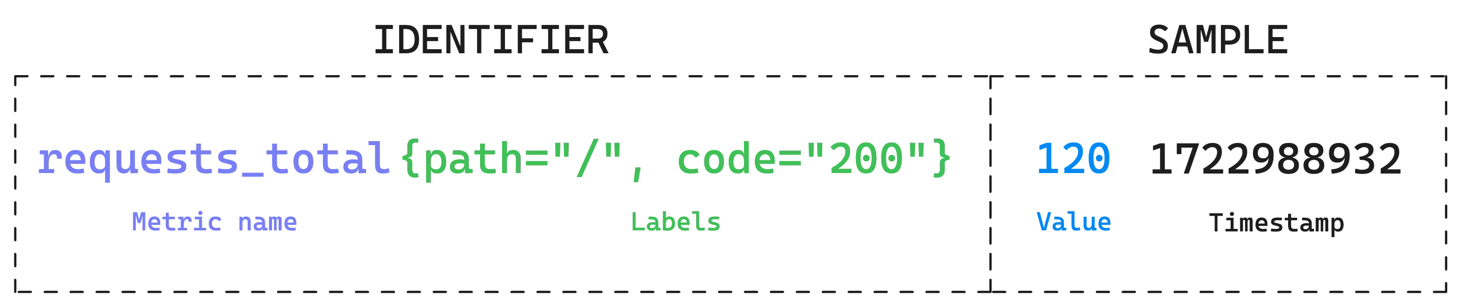
Metric structure: name, labels, value, timestamp

A metric consists of a name, labels, value, and timestamp.

That said, a metric consists of four elements: a name (a string), labels (key-value pairs), a value (a floating-point number), and a timestamp (Unix time).

Metric Name and Labels

#

Metrics can include extra details using labels, which are just key-value pairs that add context. These help break down the data in a more meaningful way. For example:

  • http_requests_total{path="/", code="200"} represents the total number of requests served at the root path / with a 200 status code.
  • http_requests_total{path="/admin", code="403"} tracks requests to /admin that resulted in a 403 (forbidden) response.

Labels aren’t always necessary. You might come across metrics without any labels when checking /metrics—the common endpoint where monitoring tools pull data from:

go_memstats_heap_alloc_bytes 1.37669232e+08
go_memstats_heap_idle_bytes 2.73235968e+08
process_open_fds 59

Even when labels aren’t explicitly shown, monitoring tools or agents often attach predefined labels in the background.

Interestingly, the metric name itself (e.g. http_requests_total) is considered a label with a special key: __name__. So, http_requests_total{path="/", code="200"} is actually the same as {__name__="http_requests_total", path="/", code="200"}.

A unique combination of a metric name and its labels forms what’s called a timeseries id. For instance, requests_total{path="/login", code="200"} and requests_total{path="/", code="200"} are two separate timeseries, even though they share the same metric name, because the path label has different values.

Every unique label value creates a new timeseries. High-cardinality labels—like IP, userID, or phoneNumber—can quickly generate an overwhelming number of timeseries, slowing down the monitoring system.

Sample

#

Each sample of a timeseries is basically a snapshot of a specific timeseries at a given moment:

  • The value is a floating-point number that represents the actual measurement—how many requests, how much CPU, etc.
  • The timestamp is when the value was recorded. If it’s not provided, monitoring tools will just use the current time when storing the sample.

Monitoring tools collect these samples from target servers at regular intervals and store them in a timeseries database. Some systems also allow applications to push metrics directly, instead of waiting for the tool to scrape them.

Metric Types

#

Monitoring systems typically don’t classify metrics into types—everything is just a measurement. That said, the idea of metric types still helps make sense of what’s being tracked.

Counter

#

A counter does exactly what you’d expect—it counts things. It only increases (or resets to zero) and never goes down.

This makes counters perfect for tracking things that continuously grow, like the number of requests hitting a server, the number of errors logged, or the total transactions processed.
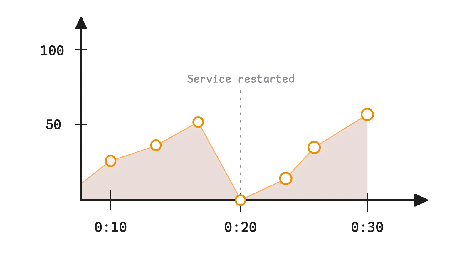
Counter

A counter only increases (or resets to zero) and never goes down.

Now, there’s a common situation where a counter might suddenly drop to zero—when a service restarts or crashes.

Fortunately, rate calculations like increase() (total increase over time) and rate() (per-second increase on average) handle this by detecting when a counter unexpectedly decreases (for example, from 200 to 0). When this happens, they assume a reset occurred and automatically add the last recorded value (200 in this case) to future counts

Therefore, even if your server crashes multiple times, the data remains smooth. You probably won’t even notice the resets in the graphs.

“How does the system know your metric is a counter? Didn’t you just say VictoriaMetrics doesn’t classify metrics into types?”.

The counter-like behavior isn’t built into the metric itself—it depends on how you query the data. Certain functions tell VictoriaMetrics to treat the data as if it were a counter:

  • increase
  • irate
  • rate

So, if you just query my_metric, you’re getting raw data—no counter reset handling, nothing fancy. But if you query rate(my_metric[5m]), VictoriaMetrics will apply counter reset detection and correction, because rate is one of those functions that expects counter behavior.

Gauge

#

Unlike counters, which only move in one direction, gauges can increase or decrease, reflecting real-time changes. This makes them useful for tracking values that fluctuate.
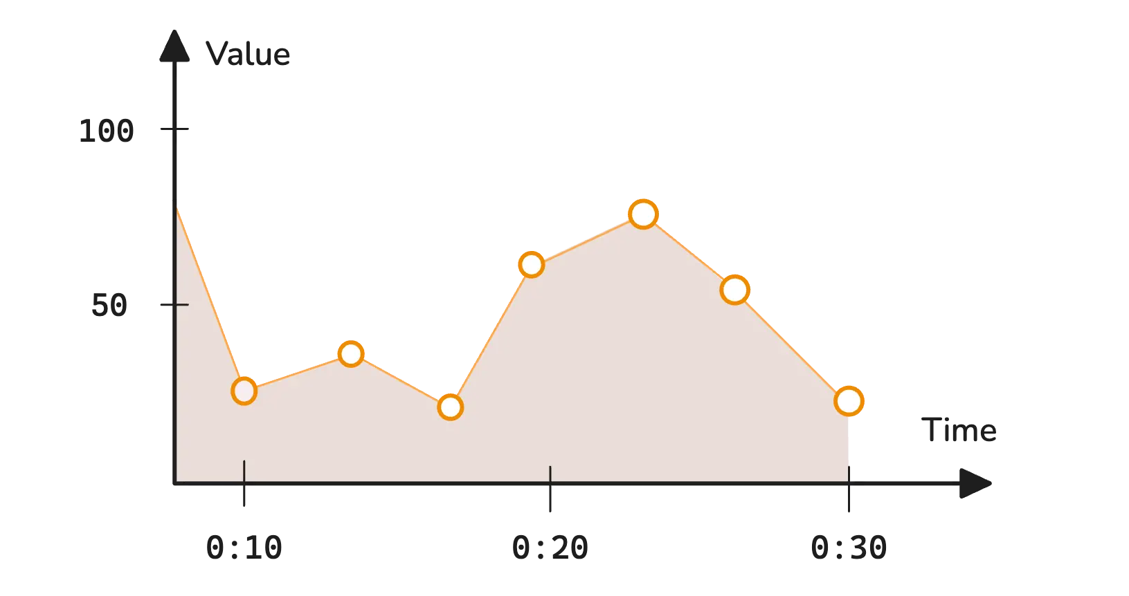
Gauges track real-time data fluctuations

Gauges track real-time data fluctuations

If you want to see how much memory is available at this moment or how busy the CPU is, a gauge gives you that snapshot. It’s not about cumulative counts—it’s about what’s happening right now.

Histogram

#

A histogram measures how values are spread across a range. In simple terms, it shows how often different values show up within certain intervals, or buckets.

To get a sense of this, take a look at this breakdown of HTTP request durations:
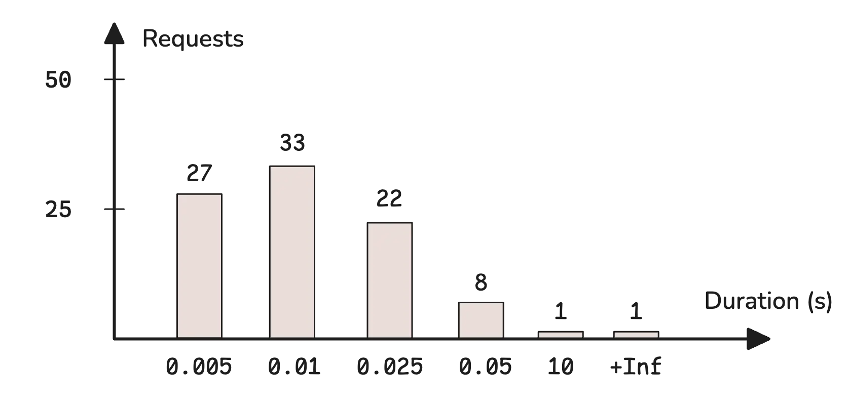
Visualizing HTTP request duration distribution

Visualizing HTTP request duration distribution

This represents different response time ranges and how many requests fall into each:

  • 0.005s bucket: 27 requests took ≤ to 0.005 seconds.
  • 0.01s bucket: 33 requests took more than 0.005s but ≤ to 0.01s.
  • 0.025s bucket: 22 requests took more than 0.01s but ≤ to 0.025s.
  • 0.05s bucket: 8 requests took more than 0.025s but ≤ to 0.05s.
  • 10s bucket: 1 request took more than 0.05s but ≤ to 10s.
  • +Inf bucket: 1 request took longer than 10s.

In monitoring, these buckets are usually defined with the le (less-or-equal) label. However, bucket values are cumulative. This means that each bucket includes all the counts from the previous ones. The chart above doesn’t reflect that directly, but a typical histogram looks more like this:
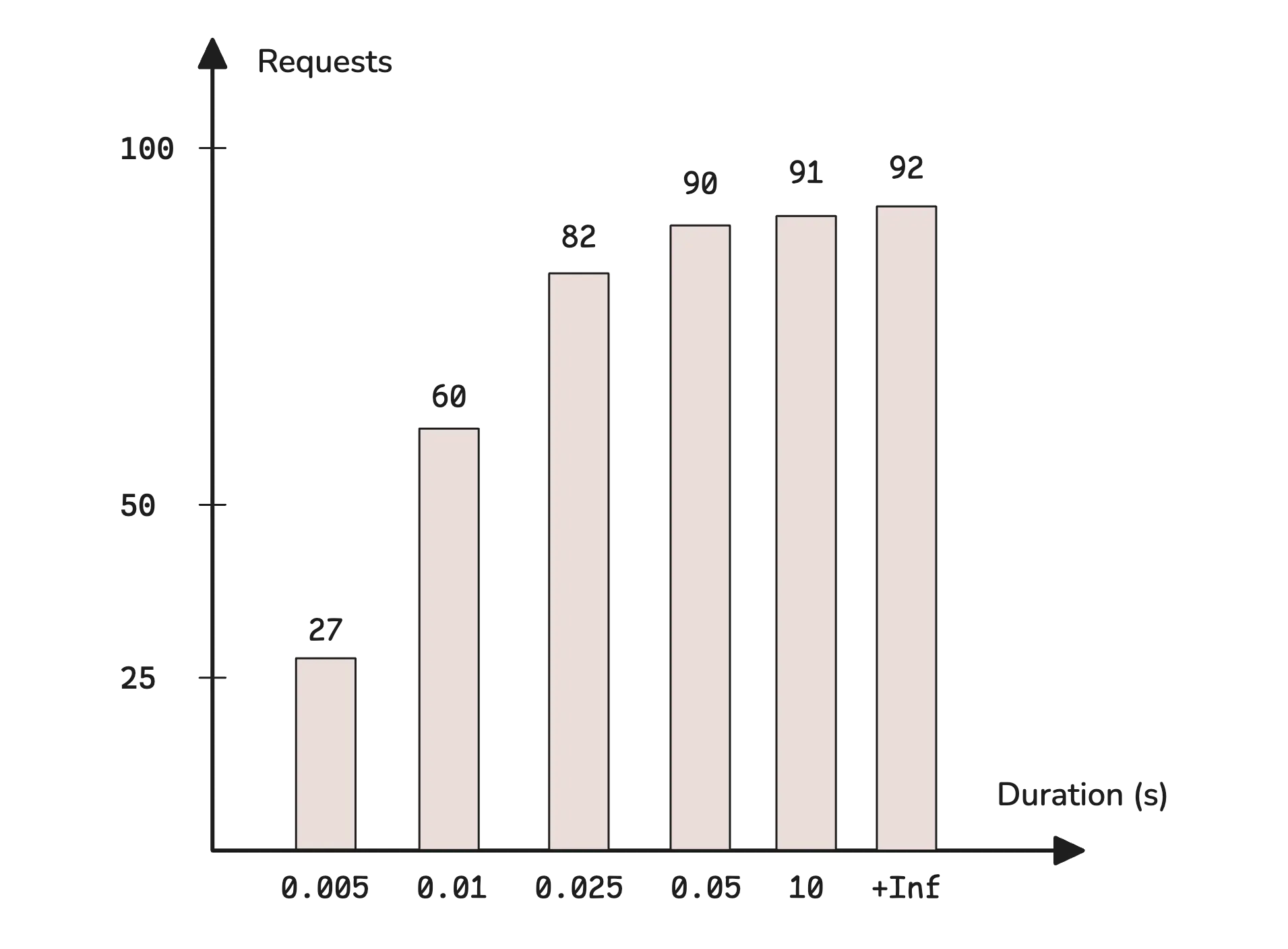
Histogram showing cumulative request counts

Histogram showing cumulative request counts

For example, http_requests_total{method="GET", le="200"} represents the total number of GET requests with a response time of 200 milliseconds or less—which also includes everything from the previous buckets (like 100ms and below).

In text format, histograms usually include three different metric suffixes:

  • _bucket: Counts how many observations fall into each range.
  • _sum: Tracks the total sum of all recorded values.
  • _count: Counts the total number of recorded observations.
http_request_duration_seconds_bucket{url="/",le="0.005"} 27
http_request_duration_seconds_bucket{url="/",le="0.01"} 60
http_request_duration_seconds_bucket{url="/",le="0.025"} 82
http_request_duration_seconds_bucket{url="/",le="0.05"} 90
http_request_duration_seconds_bucket{url="/",le="10"} 91
http_request_duration_seconds_bucket{url="/",le="+Inf"} 92
http_request_duration_seconds_sum{url="/"} 16.025
http_request_duration_seconds_count{url="/"} 92

A histogram is basically a set of counters. Looking at _count, we can see that 92 total requests were recorded. _sum tells us that the combined response time for all of them was 16.025 seconds. Most requests finished in under 0.05s.

One of the biggest advantages of histograms is that they allow percentile estimation. If you want to know how long it took to serve 95% of requests in the last 5 minutes, you can use this query:

histogram_quantile(0.95, sum(rate(http_request_duration_seconds_bucket{url="/"}[5m])) by (le))

This will tell you the response time below which 95% of requests were completed. It’s a useful way to understand performance, especially if you want to make sure that most users are getting fast responses.

Here’s how this query works, step by step:

  • rate(http_request_duration_seconds_bucket{url="/"}[5m]): Calculates the average per-second rate of requests in each bucket over the last 5 minutes.
  • sum(...) by (le): Groups all buckets with the same le value (ignoring other labels like status or method) and sums up the rates.
  • histogram_quantile(0.95, ...): Estimates the 95th percentile from the histogram data.

If you’re new to this, don’t worry. We’ll go deeper into functions later in this series.

In practice, classic histograms come with some challenges:

  • You must define bucket ranges ahead of time, but predicting accurate ranges can be difficult and may become inaccurate over time.
  • More buckets require more memory, disk space, and result in slower queries, while fewer buckets mean losing important details.
  • Two time series with different bucket ranges are not comparable and cannot be aggregated together.

To address these issues, VictoriaMetrics introduces a new histogram format: Improving Histogram Usability for Prometheus and Grafana - Aliaksandr Valialkin. Additionally, Prometheus introduced native histograms in version v2.40.0.

Summary

#

A summary works similarly to a histogram, but the key difference is where quantiles are estimated.

With histograms, data points are sorted into predefined buckets, stored as cumulative counts, and quantiles are estimated later using histogram_quantile. Summaries, on the other hand, calculate quantiles before exporting the data—right on the client side:

go_gc_duration_seconds{quantile="0"} 0.000189744
go_gc_duration_seconds{quantile="0.25"} 0.000242796
go_gc_duration_seconds{quantile="0.5"} 0.000271349
go_gc_duration_seconds{quantile="0.75"} 0.000313472
go_gc_duration_seconds{quantile="1"} 0.0021355
go_gc_duration_seconds_sum 1.519748632
go_gc_duration_seconds_count 4695

This metric tracks the duration of Go garbage collection (GC) cycles in seconds:

  • quantile="0": The shortest GC duration observed: 0.000189744 sec (189.7µs).
  • quantile="0.25": 25% of GC cycles took ≤ 0.000242796 sec (242.8µs).
  • quantile="0.5": 50% of GC cycles took ≤ 0.000271349 sec (271.3µs).
  • quantile="0.75": 75% of GC cycles took ≤ 0.000313472 sec (313.5µs).
  • quantile="1": The longest GC duration recorded: 0.0021355 sec (2.14ms).

So, most GC cycles are extremely short—just a fraction of a millisecond.

Since summaries already come with quantile labels, there’s no need to define buckets. This makes them useful when the range of values isn’t predictable.

However, you lose flexibility. Unlike histograms, summaries don’t allow percentile calculations after the fact. If you need to compute the 95th percentile later, you can’t—because it wasn’t precomputed. Summaries also can’t be aggregated across labels, meaning if you have multiple instances of an application, you can’t merge their summary data to get an overall view.

  • You can choose which quantiles a summary should track—it doesn’t have to be just 0, 0.25, 0.5, 0.75, and 1. Each quantile also comes with an associated error tolerance.
  • For example, if you configure a summary to estimate the 95th percentile (0.95 quantile) with an error margin of 0.01, it guarantees that the reported value is within ±1% of the actual 95th percentile.
  • This error margin exists because storing every single observation to compute exact quantiles would be too resource-intensive. Instead, summaries use algorithms that approximate quantiles within the allowed error range. A summary estimating the 95th percentile with a 1% error margin will require more resources than one allowing a 5% margin.

Naming Conventions

#

The most important rule in naming metrics is to keep them readable, descriptive, and clear. When you have hundreds or even thousands of metrics, you want to pick them wisely—without wasting time trying to figure out what each one actually represents.

That said, there are a few conventions for naming metrics and labels. These aren’t strict rules, but following them keeps things consistent:

  • Use snake_case: Metric and label names should be in snake_case, and free of special characters.
  • Label value: There aren’t any strict restrictions here, but it’s best to avoid spaces; prefer a dash (-) instead. For example, env="prod-us-west" is better than env="prod us west".
  • Metric name prefix: A prefix usually describes the component or service. Some common ones include http_, go_, node_, mysql_, redis_, etc.
  • Metric name suffix: The suffix usually indicates either the metric type or the base unit of the measurement (typically in plural form).
    • Metric type is often reflected in the suffix, such as _total and _count for counters. It can be combined with base units, e.g. _bytes_total, _seconds_total.
    • Base units are commonly used in gauges, such as _bytes, _errors, and _seconds. It’s best to stick to base units—prefer seconds over milliseconds.
  • No redundant label names: If the metric name already provides context, there’s no need to repeat it in the labels. Instead of http_requests_total{http_status="200"}, just use status="200".
  • Consistent naming: If one metric uses service="auth", don’t use app="auth-service" in another. Stick to the same structure.

For more details, check out Prometheus’s Metric and label naming.

Stay Connected

#

If you spot anything that’s outdated or have questions, don’t hesitate to reach out. You can drop me a DM on X(@func25) or VictoriaMetrics’ Slack.

Who We Are

#

If you want to monitor your services, track metrics, and see how everything performs, you might want to check out VictoriaMetrics. It’s a fast, open-source, and cost-saving way to keep an eye on your infrastructure.