This is a guest post by Shayan, an International Grandmaster on Codeforces and a PhD Candidate at the University of Maryland.

In this post Shayan will share top 7 graph algorithms to know if you are preparing for coding interviews.

Graphs come up in about 35-40% of coding interviews at major tech companies because so many real systems are graphs: social networks, map routing, dependency chains, web crawlers. If you don’t know core graph patterns, you’ll struggle in the interview.

I’ve seen candidates get stuck on problems like “Number of Islands” simply because they hadn’t practiced basic grid traversal. These problems become straightforward once you know the patterns.

In this post, I’ll show you 7 graph algorithms that cover about 85% of graph-related interview questions. For each one, you’ll learn what it does, when to use it, how it works, and which LeetCode problems to practice.

This post is based on Repovive's Graph Theory roadmap. Let's get into it.

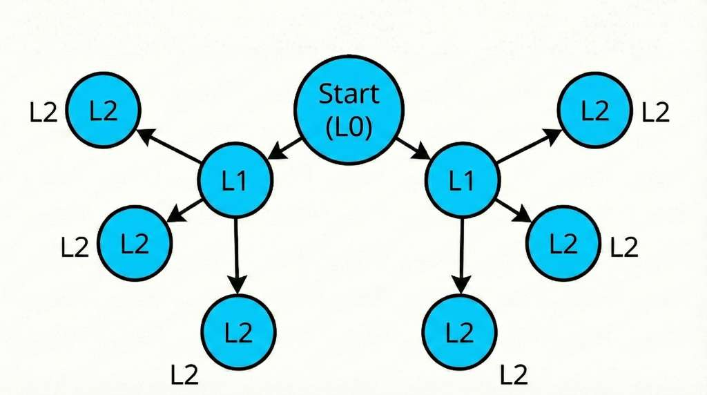
What it is: BFS explores a graph level by level. It visits every node at distance 1 from the start, then distance 2, then distance 3, and so on.

Use BFS when the problem is naturally about layers or minimum steps:

• Finding the shortest path in an unweighted graph

• Level-order traversal

• Finding all nodes within K distance

• Any problem that asks for “minimum steps” or “shortest path” without weights

BFS uses a queue. You start by adding the source node. Then you repeat: remove the front node, process it, and add all its unvisited neighbors to the back of the queue.

The queue enforces the level-by-level order. By the time you reach a node, you’ve visited all closer nodes first. This guarantees the first path you find is the shortest.

queue = [start]
visited = {start}

while queue is not empty:
    node = queue.pop_front()
    for neighbor in node.neighbors:
        if neighbor not in visited:
            visited.add(neighbor)
            queue.push_back(neighbor)

BFS works well on 2D grids.

Think of grids like this:

• Each cell is a node

• Its neighbors are usually up, down, left, right (sometimes diagonals too)

Problems like “Number of Islands” and “Rotting Oranges” are grid-based BFS.

For flood fill, you start at a cell and spread to all connected cells matching a condition. You stop at boundaries or cells that don’t match. This is the algorithm behind the paint bucket tool in image editors.

• Shortest Path in Binary Matrix (Medium)

• Rotting Oranges (Medium)

• Number of Islands (Medium)

• 01 Matrix (Medium)

• Word Ladder (Hard)

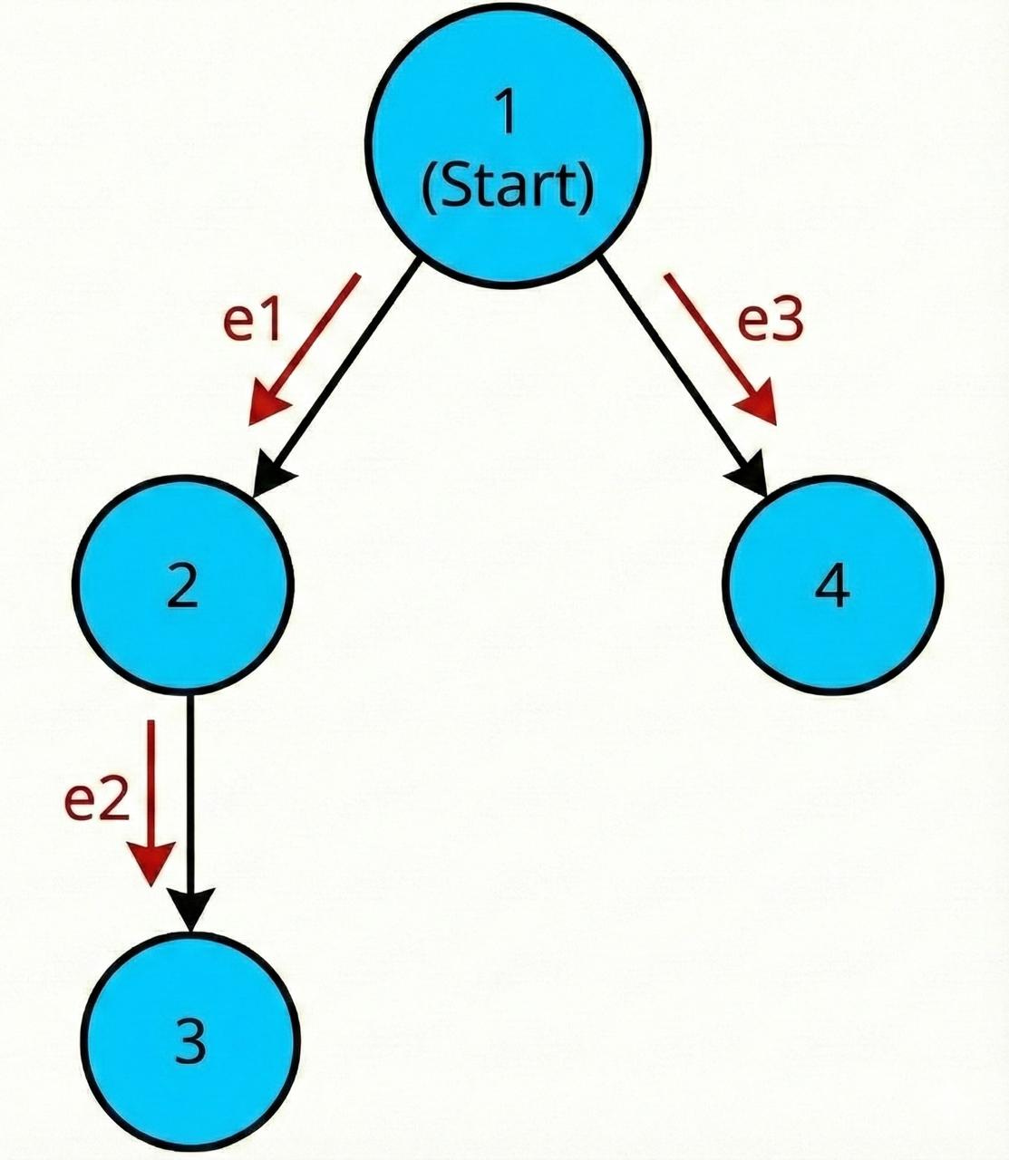
What it is: DFS explores a graph as deep as possible before it backtracks. If a node has multiple neighbors, DFS fully explores the first neighbor’s branch, then returns and tries the next.

DFS is the right tool when you care about reachability, structure, or exhaustive exploration, not minimum distance:

• Detecting cycles

• Finding connected components

• Path finding (when you don’t need the shortest path)

• Backtracking problems

• Tree traversals

A good mental model is a maze.

You choose a path, keep walking, and mark where you’ve been. When you hit a dead end, you backtrack to the last fork and try a different direction.

DFS uses a stack:

• Either an explicit stack you manage yourself

• Or recursion, which uses the call stack implicitly

Because the “most recent” node is processed next, DFS naturally pushes deeper into the graph.

function dfs(node):
    if node in visited:
        return
    visited.add(node)

    for neighbor in node.neighbors:
        dfs(neighbor)

DFS is one of the most common ways to detect cycles, but the exact rule depends on the graph type (directed vs undirected graphs).

For undirected graphs: if you reach a visited node that isn’t your immediate parent, you’ve found a cycle.

For directed graphs: you use three states (unvisited, in-progress, completed). If you reach an in-progress node, you’ve found a back edge, which means a cycle.

// Directed graph cycle detection
state = [UNVISITED] * n

function hasCycle(node):
    state[node] = IN_PROGRESS

    for neighbor in node.neighbors:
        if state[neighbor] == IN_PROGRESS:
            return true  // cycle found
        if state[neighbor] == UNVISITED:
            if hasCycle(neighbor):
                return true

    state[node] = COMPLETED
    return false

Practice these LeetCode problems:

• Clone Graph (Medium)

• Number of Provinces (Medium)

• Max Area of Island (Medium)

• Course Schedule (Medium)

• All Paths From Source to Target (Medium)

What it is: Dijkstra’s Algorithm finds the shortest path in a weighted graph where all edge weights are non-negative. Unlike BFS, it works when edges have different costs.

Reach for Dijkstra when you see weights and the question is about minimum cost:

• Shortest path with weighted edges

• Navigation and routing (Google Maps)

• Network routing with latency costs

• Any problem mentioning “minimum cost path”

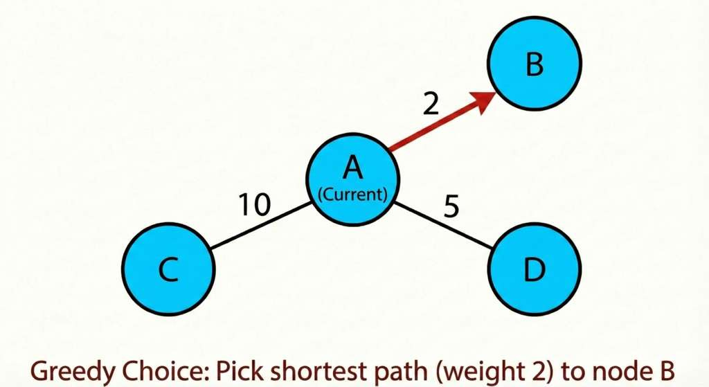
BFS doesn’t work on weighted graphs because one step doesn’t equal one unit of distance. A direct path might cost 10 while a two-step path costs 2.

Dijkstra fixes this by always expanding the currently cheapest known node first:

• Maintain dist[node] = best known distance from the source

• Use a min-heap / priority queue keyed by distance

• Pop the node with the smallest distance, then relax its edges

If the graph has only non-negative weights, the first time a node is popped with its best distance, that distance is final.

dist = [infinity] * numNodes
dist[source] = 0
pq = [(0, source)]  // (distance, node)

while pq is not empty:
    d, node = pq.pop_min()

    if d > dist[node]:
        continue  // found a better path already

    for (neighbor, weight) in node.edges:
        newDist = d + weight
        if newDist < dist[neighbor]:
            dist[neighbor] = newDist
            pq.push((newDist, neighbor))

You have n network nodes. You’re given travel times as directed edges (u, v, w) where w is the time. You send a signal from node k. How long until all nodes receive it?

To solve this, you run Dijkstra from node k. Your answer is the maximum distance among all reachable nodes. If any node is unreachable, you return -1.

• Network Delay Time (Medium)

• Path with Minimum Effort (Medium)

• Cheapest Flights Within K Stops (Medium)

• Swim in Rising Water (Hard)

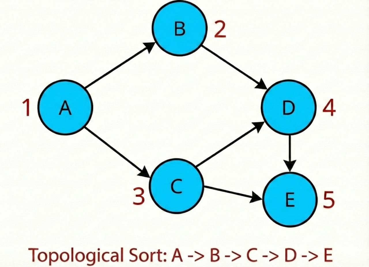
What it is: Topological sort orders nodes in a Directed Acyclic Graph (DAG) so that for every edge u → v, node u appears before node v. In plain terms: it gives you an execution order that respects dependencies. That’s why it shows up so often in scheduling-style problems.

Topological sort is the default pattern when you see dependency language:

• Course scheduling with prerequisites

• Build systems and dependency resolution

• Task ordering

• Any problem that mentions “prerequisites” or “dependencies”

Kahn’s algorithm is the BFS-style way to do topological sorting.

Key idea: A node’s in-degree is the number of edges pointing to it. If a node has in-degree 0, it has no dependencies and you can process it.

You start by adding all nodes with in-degree 0 to a queue. You process them one by one. When you process a node, you decrement the in-degree of its neighbors. If a neighbor’s in-degree drops to 0, you add it to the queue.

If you process all nodes, you have a valid topological order. If the queue empties before you’ve processed all nodes, you’ve found a cycle.

inDegree = count incoming edges for each node
queue = all nodes with inDegree 0
result = []

while queue is not empty:
    node = queue.pop()
    result.append(node)

    for neighbor in node.outgoing:
        inDegree[neighbor] -= 1
        if inDegree[neighbor] == 0:
            queue.push(neighbor)

if len(result) < numNodes:
    return "cycle detected"

You have numCourses courses. Some have prerequisites: [0, 1] means you take course 1 before course 0. You need to return any valid order to finish all courses, or an empty array if impossible.

To solve this, you build a directed graph where edge b→a means “take b before a”. Then run Kahn’s algorithm. If you can’t process all courses, you’ve found a cyclic dependency.

• Course Schedule (Medium)

• Course Schedule II (Medium)

• Alien Dictionary (Hard)

• Parallel Courses (Medium)

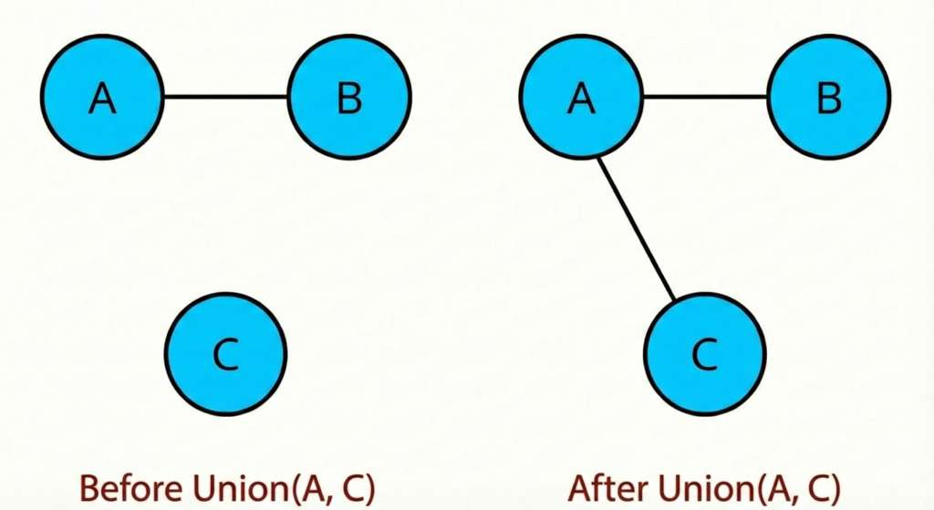
What it is: Union-Find is a data structure for tracking a collection of elements split into disjoint (non-overlapping) sets. It supports two core operations:

• find(x): which set does x belong to?

• union(x, y): merge the sets containing x and y

Once you have these, you can answer connectivity questions like “are these two nodes connected?” efficiently.

Union-Find shines when you’re adding connections over time and need fast connectivity checks:

• Dynamic connectivity queries

• Detecting cycles in undirected graphs

• Kruskal’s MST algorithm

• Grouping elements as edges are added

Each set has a leader (representative). Two elements are in the same set if they have the same leader. You store a parent array where parent[i] points to i’s parent. The root is the leader (where parent[i] = i).

To make operations extremely fast in practice, Union-Find uses two standard optimizations:

1. Path compression: When you find the leader, you make each node on the path point directly to the leader.

2. Union by rank/size: When merging two sets, attach the smaller tree under the larger one to keep trees shallow.

parent = [0, 1, 2, ..., n-1]  // each node is its own leader
rank = [0] * n

function find(x):
    if parent[x] != x:
        parent[x] = find(parent[x])  // path compression
    return parent[x]

function union(x, y):
    px, py = find(x), find(y)
    if px == py:
        return false  // already connected

    if rank[px] < rank[py]:
        parent[px] = py
    else if rank[px] > rank[py]:
        parent[py] = px
    else:
        parent[py] = px
        rank[px] += 1

    return true

You have a graph that started as a tree (connected, no cycles), then one edge was added. You need to find the edge that can be removed to restore the tree.

To solve this using union find, process edges one by one. For each edge (u, v), you check if u and v are already connected using find(). If yes, this edge creates a cycle. If no, you union them. The first edge that connects already-connected nodes is your answer.

• Redundant Connection (Medium)

• Number of Provinces (Medium)

• Accounts Merge (Medium)

• Satisfiability of Equality Equations (Medium)

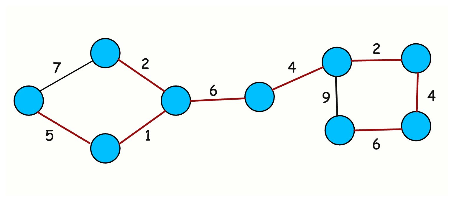
What it is: A spanning tree connects all nodes in a graph using exactly n-1 edges with no cycles. The minimum spanning tree is the one with the smallest total edge weight.

MST comes up whenever you need to connect a set of nodes with minimum total cost:

• Connecting all nodes with minimum cost

• Network design (cables, roads, pipelines)

• Clustering algorithms

• Approximation algorithms for NP-hard problems

Kruskal’s is the most common MST approach in interviews because it’s simple and pairs naturally with Union-Find.

You sort all edges by weight. You process them in order. For each edge, you use Union-Find to check if it connects two different components. If yes, you add it to the MST. If no, you skip it to avoid a cycle.

edges.sort(by weight)
mst = []
uf = UnionFind(n)

for edge in edges:
    u, v, weight = edge
    if uf.find(u) != uf.find(v):
        uf.union(u, v)
        mst.append(edge)

    if len(mst) == n - 1:
        break

return mst

You’re given points on a 2D plane. The cost to connect two points is their Manhattan distance. You return the minimum cost to connect all points.

To solve this, you treat each pair of points as a potential edge. Generate all edges, sort by weight, and run Kruskal’s. The MST gives you the minimum total cost.

• Min Cost to Connect All Points (Medium)

• Connecting Cities With Minimum Cost (Medium)

• Find Critical and Pseudo-Critical Edges in MST (Hard)

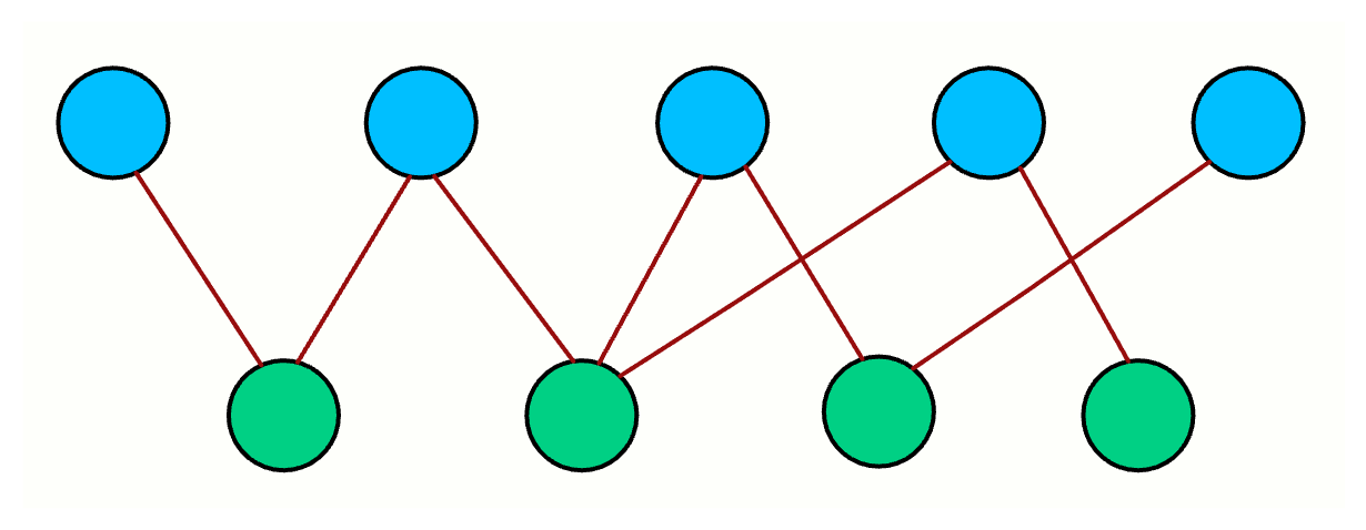
What it is: A graph is bipartite if you can split its nodes into two groups such that every edge connects nodes from different groups. No edge is allowed within the same group.

A simple way to remember it: Can you 2-color the graph so that no two adjacent nodes share the same color?

Bipartite checks appear whenever the problem is about dividing things into two compatible sets:

• Team or group assignments

• Matching problems

• Checking for odd-length cycles (a graph is bipartite if and only if it has no odd-length cycles)

• Scheduling with conflicts

You can use BFS or DFS to try 2-coloring the graph.

Pick a start node and assign it color 0. Assign all its neighbors color 1. Assign their neighbors color 0. Continue alternating.

If you ever find an edge where both endpoints have the same color, the graph is not bipartite.

color = [-1] * n  // uncolored

function isBipartite(start):
    queue = [start]
    color[start] = 0

    while queue is not empty:
        node = queue.pop()
        for neighbor in node.neighbors:
            if color[neighbor] == -1:
                color[neighbor] = 1 - color[node]
                queue.push(neighbor)
            else if color[neighbor] == color[node]:
                return false

    return true

You’re given an undirected graph. You return true if it’s bipartite.

Because the graph may be disconnected, run BFS/DFS from every uncolored node:

• Start a new traversal, try to 2-color that component

• If any component fails, return false

• If all components succeed, the graph is bipartite

• Is Graph Bipartite? (Medium)

• Possible Bipartition (Medium)

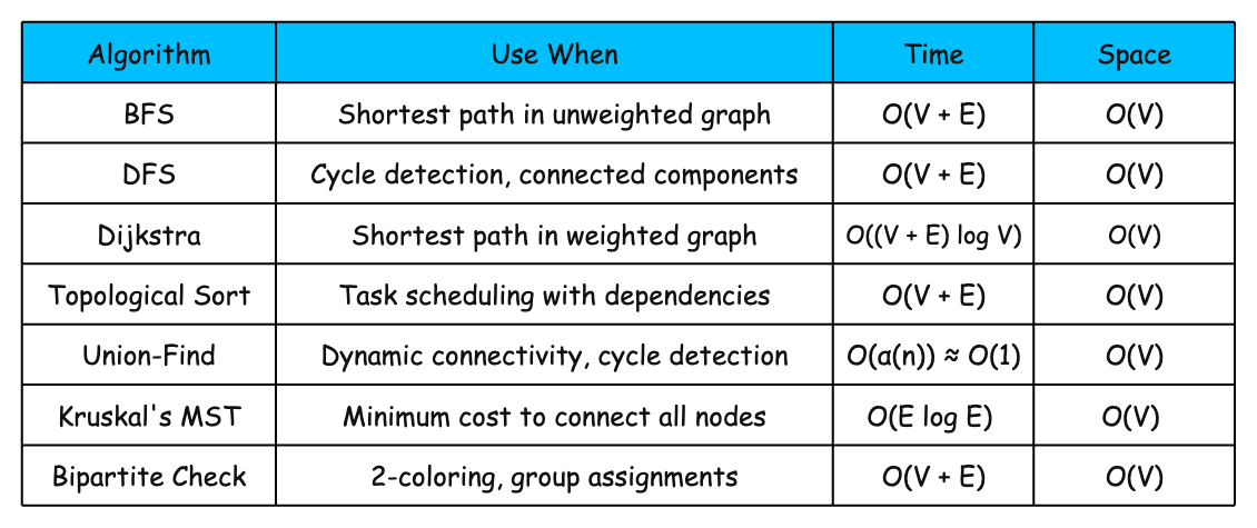
You now have 7 algorithms that cover most graph problems in coding interviews. Here’s how to retain them:

1. Practice in order. Start with BFS and DFS. They’re the foundation the others build on.

2. Match patterns to algorithms. “Shortest path” without weights → BFS. “Prerequisites” or “dependencies” → topological sort. “Minimum cost to connect” → MST.

3. Implement from scratch. Don’t just read the code. Write it yourself. Debug it. That’s how you learn.

4. Practice with time limits. In interviews, you have 20-30 minutes per problem. Get comfortable working under that constraint.

For a structured approach to learn, feel free to take a look at our roadmaps. It covers these algorithms plus topics like Strongly Connected Components, Lowest Common Ancestor, and Network Flow.