马尔科夫链蒙特卡洛方法和吉布斯采样
MCMC and Gibbs Sampling
分类: 机器学习 / 字数: 3544 / 标签: 马尔科夫链蒙特卡洛方法, MCMC, 吉布斯采样, Gibbs Sampling
蒙特卡罗方法 (Monte Carlo) 也称为统计模拟方法,是于 20 世纪 40 年代由冯·诺伊曼,斯塔尼斯拉夫·乌拉姆和尼古拉斯·梅特罗波利斯在洛斯阿拉莫斯国家实验室为核武器计划工作时 (曼哈顿计划) 发明。因为乌拉姆的叔叔经常在摩纳哥的蒙特卡罗赌场输钱,该方法被定名为蒙特卡罗方法。蒙特卡罗方法是以概率为基础的方法,与之对应的是确定性算法。
蒙特卡罗方法最早可以追述到 18 世纪的布丰投针问题,该方法通过一个平行且等距木纹铺成的地板,随意抛一支长度比木纹之间距离小的针,求针和其中一条木纹相交的概率的方法得出了一个求 $\pi$ 的蒙特卡罗方法。我们通过另一种方式使用蒙特卡罗方法计算圆周率 $\pi$,对于一个边长为 $2r$ 的正方形,其内切圆的半径即为 $r$,因此圆形的面积 $A_c$ 与正方形的面积 $A_s$ 的比值为
$$ \dfrac{A_c}{A_s} = \dfrac{\pi r^2}{\left(2r\right)^2} = \dfrac{\pi}{4} $$
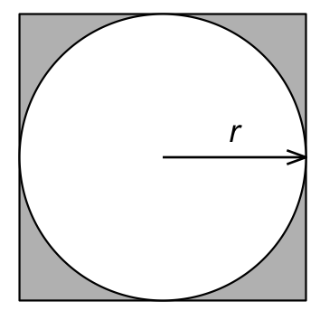
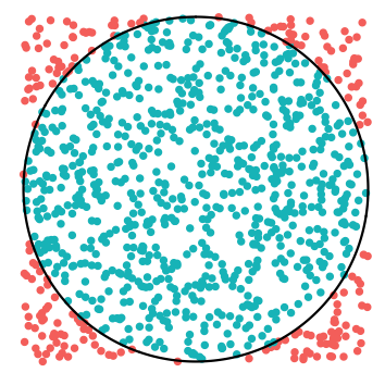
如果我们在矩形内随机的生成均匀分布的点,则在圆内的点的个数的占比即为 $\dfrac{\pi}{4}$,因此通过模拟即可求出 $\pi$ 的近似值
library(tidyverse)

# 圆的中心点和半径
r <- 2
center_x <- r
center_y <- r

# 距离公式
distance <- function(point_x, point_y, center_x, center_y) {
    sqrt((point_x - center_x)^2 + (point_y - center_y)^2)
}

# 点生成器
points_generator <- function(size) {
    set.seed(112358)
    points_x <- runif(size, min = 0, max = 2*r)
    points_y <- runif(size, min = 0, max = 2*r)

    tibble(
        x = points_x,
        y = points_y,
        in_cycle = ifelse(
            distance(points_x, points_y, center_x, center_y) > r, 0, 1)
    )
}

# 点的个数
sizes <- c(1000, 10000, 100000, 1000000, 10000000)

# 估计的 PI 值
estimated_pi <- sapply(sizes, function(size) {
    points <- points_generator(size)
    sum(points$in_cycle) * 4 / size
})
print(estimated_pi)
# [1] 3.184000 3.146400 3.137880 3.143140 3.141889
模拟 $1000$ 个随机点的结果如图所示
对于简单的分布 $p\left(x\right)$,我们可以相对容易的生成其样本,但对于复杂的分布或高维的分布,样本的生成就比较困难了1,例如:
$p\left(x\right) = \dfrac{\tilde{p}\left(x\right)}{\int\tilde{p}\left(x\right) dx}$,其中 $\tilde{p}\left(x\right)$ 是可以计算的,而分母中的积分是无法显式计算的。$p\left(x, y\right)$ 是一个二维分布函数,函数本身计算很困难,但其条件分布 $p\left(x | y\right)$ 和 $p\left(y | x\right)$ 计算相对简单。对于高维情况 $p\left(\boldsymbol{x}\right)$,这种情况则更加明显。这时候则需要更加复杂的模拟方法来生成样本了。
马尔可夫过程 (Markov Process) 是因俄国数学家安德雷·安德耶维齐·马尔可夫 (Андрей Андреевич Марков) 而得名一个随机过程,在该随机过程中,给定当前状态和过去所有状态的条件下,其下一个状态的条件概率分布仅依赖于当前状态,通常具备离散状态的马尔科夫过程称之为马尔科夫链 (Markov Chain)。因此,马尔科夫链可以理解为一个有限状态机,给定了当前状态为 $s_i$ 时,下一时刻状态为 $s_j$ 的概率,不同状态之间变换的概率称之为转移概率。下图描述了 3 个状态 $S_a, S_b, S_c$ 之间转换状态的马尔科夫链。

对于马尔科夫链,我们设 $X_t$ 表示 $t$ 时刻随机变量 $X$ 的取值,则马尔科夫链可以表示为
$$ P\left(X_{t+1} = s_j | X_0 = s_{i0}, X_1 = s_{i1}, ..., X_t = s_i\right) = P\left(X_{t+1} | X_t = s_i\right) $$
其中,$s_{i0}, s_{i1}, ..., s_i, s_j$ 为随机变量 $X$ 可能的状态。则定义从一个状态 $s_i$ 到另一个状态 $s_j$ 的转移概率为
$$ P\left(i \to j\right) = P_{ij} = P\left(X_{t+1} | X_t = s_i\right) $$
设 $\pi_{k}^{\left(t\right)}$ 表示随机变量 $X$ 在 $t$ 时刻取值为 $s_k$ 的概率,则 $X$ 在 $t+1$ 时刻取值为 $s_i$ 的概率为
$$ \begin{equation} \begin{split} \pi_{i}^{\left(t+1\right)} &= P\left(X_{t+1} = s_i\right) \\ &= \sum_{k}{P\left(X_{t+1} = s_i | X_t = s_k\right) \cdot P\left(X_t = s_k\right)} \\ &= \sum_{k}{P_{ki} \cdot \pi_{k}^{\left(t\right)}} \end{split} \end{equation} $$
我们通过一个例子来理解一下马尔科夫链,我们使用 LDA 数学八卦1一文中的例子,对于人口,我们将其经济状况分为 3 类:下层,中层和上层,其父代到子代收入阶层的转移情况如表所示
| 父代阶层\子代阶层 | 下层 | 中层 | 下层 |
|---|---|---|---|
| 下层 | 0.65 | 0.28 | 0.07 |
| 中层 | 0.15 | 0.67 | 0.18 |
| 上层 | 0.12 | 0.36 | 0.52 |
我们利用矩阵的形式表示转移概率
$$ P = \left\lgroup \begin{array}{cccc} P_{11} & P_{12} & \cdots & P_{1n} \\ P_{21} & P_{22} & \cdots & P_{2n} \\ \vdots & \vdots & & \vdots \\ P_{n1} & P_{n2} & \cdots & P_{nn} \end{array} \right\rgroup $$
则
$$ \pi^{\left(t+1\right)} = \pi^{\left(t\right)} P $$
假设初始概率分布为 $\pi_0 = \left(0.21, 0.68, 0.11\right)$,则计算前 $n$ 代人的阶层分布情况如下
# 转移矩阵
p <- matrix(c(0.65, 0.28, 0.07,
              0.15, 0.67, 0.18,
              0.12, 0.36, 0.52),
            3, 3, byrow = T)
# 初始概率
pi <- matrix(c(0.21, 0.68, 0.11), 1, 3, byrow = T)

# 迭代变化
for (i in 1:10) {
    pi_current <- pi[i, ]
    pi_next <- pi_current %*% p
    pi <- rbind(pi, pi_next)
}

colnames(pi) <- c('下层', '中层', '上层')
rownames(pi) <- 0:10
print(pi)
#         下层      中层      上层
# 0  0.2100000 0.6800000 0.1100000
# 1  0.2517000 0.5540000 0.1943000
# 2  0.2700210 0.5116040 0.2183750
# 3  0.2784592 0.4969956 0.2245452
# 4  0.2824933 0.4917919 0.2257148
# 5  0.2844752 0.4898560 0.2256688
# 6  0.2854675 0.4890974 0.2254351
# 7  0.2859707 0.4887828 0.2252465
# 8  0.2862280 0.4886450 0.2251270
# 9  0.2863602 0.4885817 0.2250581
# 10 0.2864283 0.4885515 0.2250201
可以看出,从第 7 代人开始,分布就基本稳定下来了,如果将初值概率换成 $\pi_0 = \left(0.75, 0.15, 0.1\right)$,结果会是如何呢?
pi <- matrix(c(0.75, 0.15, 0.1), 1, 3, byrow = T)

for (i in 1:10) {
    pi_current <- pi[i, ]
    pi_next <- pi_current %*% p
    pi <- rbind(pi, pi_next)
}

colnames(pi) <- c('下层', '中层', '上层')
rownames(pi) <- 0:10
print(pi)
#         下层      中层      上层
# 0  0.7500000 0.1500000 0.1000000
# 1  0.5220000 0.3465000 0.1315000
# 2  0.4070550 0.4256550 0.1672900
# 3  0.3485088 0.4593887 0.1921025
# 4  0.3184913 0.4745298 0.2069789
# 5  0.3030363 0.4816249 0.2153388
# 6  0.2950580 0.4850608 0.2198812
# 7  0.2909326 0.4867642 0.2223032
# 8  0.2887972 0.4876223 0.2235805
# 9  0.2876912 0.4880591 0.2242497
# 10 0.2871181 0.4882830 0.2245989
可以看出从第 9 代人开始,分布又变得稳定了,这也就是说分布收敛情况是不随初始概率分布 $\pi_0$ 的变化而改变的。则对于具有如下特征的马尔科夫链
则这样的马尔科夫链,无论 $\pi_0$ 取值如何,最终随机变量的分布都会收敛于 $\pi^*$,即
$$ \pi^* = \lim_{t \to \infty}{\pi^{\left(0\right)} \boldsymbol{P}^t} $$
$\pi^*$ 称之为这个马尔科夫链的平稳分布。
构造一个转移矩阵为 $P$ 的马尔科夫链,如果其能收敛到平稳分布 $p\left(x\right)$,则可以从任意一个状态 $x_0$ 出发,得到一个状态转移序列 $x_0, x_1, ..., x_n, x_{n+1}, ...$,如果马尔科夫链在第 $n$ 部收敛,我们就可以得到服从分布 $p\left(x\right)$ 的样本 $x_n, x_{n+1}, ...$。因此,利用马尔科夫链的平稳性生成数据的样本的关键就在于如何构造一个状态转移矩阵 $P$,使得其平稳分布为 $p\left(x\right)$。
如果对于任意的 $i, j$,马尔科夫链的转移矩阵 $P$ 和分布 $\pi\left(x\right)$ 满足
$$ \pi\left(i\right) P_{ij} = \pi\left(j\right) P_{ji} $$
则称 $\pi\left(x\right)$ 为马尔科夫链的平稳分布,这称为细致平稳条件。对于一个马尔科夫链,通常情况下
$$ p\left(i\right) q\left(i, j\right) \neq p\left(j\right) q\left(j, i\right) $$
其中 $p\left(i, j\right)$ 表示状态从 $i$ 转移到 $j$ 的概率。因此,为了构造满足细致平稳条件,我们引入一个接受概率 $\alpha\left(i, j\right)$,使得
$$ p\left(i\right) q\left(i, j\right) \alpha\left(i, j\right) = p\left(j\right) q\left(j, i\right) \alpha\left(j, i\right) $$
最简单的,我们取
$$ \alpha\left(i, j\right) = p\left(j\right) q\left(j, i\right), \alpha\left(j, i\right) = p\left(i\right) q\left(i, j\right) $$
即可保证细致平稳性。通过引入接受概率,我们将原始的马尔科夫链改造为具有新的转移矩阵的马尔科夫链。在原始马尔科夫链上以概率 $q\left(i, j\right)$ 从状态 $i$ 转移到状态 $j$ 时,我们以概率 $\alpha\left(i, j\right)$ 接受这个转移,因此在新的马尔科夫链上的转移概率为 $q\left(i, j\right) \alpha\left(i, j\right)$。在新的马尔科夫链转移的过程中,如果接受概率 $\alpha\left(i, j\right)$ 过小,则可能导致存在大量的拒绝转移,马尔科夫链则很难收敛到平稳分布 $p\left(x\right)$,因此我们对 $\alpha\left(i, j\right), \alpha\left(j, i\right)$ 进行同比例放大,将其中较大的数放大至 $1$,则可以增加接受跳转的概率,从而更快的收敛到平稳分布。因此,我们可以取
$$ \alpha\left(i, j\right) = \min \left\lbrace\dfrac{p\left(j\right) q\left(j, i\right)}{p\left(i\right) q\left(i, j\right)}, 1\right\rbrace $$
这样我们就得到了 Metropolis-Hastings 算法
\begin{algorithm}
\caption{Metropolis-Hastings 算法}
\begin{algorithmic}
\STATE $X_0 \gets x_0$
\FOR{$t = 0, 1, 2, ...$}
    \STATE $X_t = x_t$
    \STATE sample $y \sim q\left(x | x_t\right)$
    \STATE sample $u \sim Uniform[0, 1]$
    \IF{$u < \alpha\left(x_t, y\right) = \min\left\lbrace\dfrac{p\left(j\right) q\left(j, i\right)}{p\left(i\right) q\left(i, j\right)}, 1\right\rbrace$}
        \STATE $X_{t+1} \gets y$
    \ELSE
        \STATE $X_{t+1} \gets x_t$
    \ENDIF
\ENDFOR
\end{algorithmic}
\end{algorithm}
对于 Metropolis-Hastings 算法,由于存在接受跳转概率 $\alpha < 1$,因此为了提高算法效率,我们尝试构建一个转移矩阵,使得 $\alpha = 1$。以二维情形为例,对于概率分布 $p\left(x, y\right)$,考虑两个点 $A\left(x_1, y_1\right)$ 和 $B\left(x_1, y_2\right)$
$$ \begin{equation} \begin{split} p\left(x_1, y_1\right) p\left(y_2 | x_1\right) &= p\left(x_1\right) p\left(y_1 | x_1\right) p\left(y_2 | x_1\right) \\ p\left(x_1, y_2\right) p\left(y_1 | x_1\right) &= p\left(x_1\right) p\left(y_2 | x_1\right) p\left(y_1 | x_1\right) \end{split} \end{equation} $$
可得
$$ \begin{equation} \begin{split} p\left(x_1, y_1\right) p\left(y_2 | x_1\right) &= p\left(x_1, y_2\right) p\left(y_1 | x_1\right) \\ p\left(A\right) p\left(y_2 | x_1\right) &= p\left(B\right) p\left(y_1 | x_1\right) \end{split} \end{equation} $$
可以得出在 $x = x_1$ 上任意两点之间进行转移均满足细致平稳条件,同理可得在 $y = y_1$上也满足。因此,对于二维情况,我们构建满足如下调价的概率转移矩阵 $Q$
$$ \begin{equation} \begin{split} &Q\left(A \to B\right) = p\left(y_B | x_1\right), \text{for} \ x_A = x_B = x_1 \\ &Q\left(A \to C\right) = p\left(x_C | y_1\right), \text{for} \ y_A = y_C = y_1 \\ &Q\left(A \to D\right) = 0, \text{others} \end{split} \end{equation} $$
则对于平面上任意两点 $X, Y$ 满足细致平稳条件
$$ p\left(X\right) Q\left(X \to Y\right) = p\left(Y\right) Q\left(Y \to X\right) $$
对于如上过程,我们不难推广到多维情况,将 $x_1$ 变为多维情形 $\boldsymbol{x_1}$,容易验证细致平稳条件依旧成立。
$$ p\left(\boldsymbol{x_1}, y_1\right) p\left(y_2 | \boldsymbol{x_1}\right) = p\left(\boldsymbol{x_1}, y_2\right) p\left(y_1 | \boldsymbol{x_1}\right) $$
对于 $n$ 维的情况,通过不断的转移得到样本 $\left(x_1^{\left(1\right)}, x_2^{\left(1\right)}, ..., x_n^{\left(1\right)}\right)$, $\left(x_1^{\left(2\right)}, x_2^{\left(2\right)}, ..., x_n^{\left(2\right)}\right)$, …,当马尔科夫链收敛后,后续得到的样本即为 $p\left(x_1, x_2, ..., x_n\right)$ 的样本,收敛之前的这一阶段我们称之为 burn-in period。在进行转移的时候,坐标轴轮换的采样方法并不是必须的,可以在坐标轴轮换中引入随机性。至此,我们就得到了吉布斯采样算法
\begin{algorithm}
\caption{Gibbs Sampling 算法}
\begin{algorithmic}
\STATE initialize $x^{\left(0\right)}, \text{for} \ i = 1, 2, ..., n$
\FOR{$t = 0, 1, 2, ...$}
    \STATE $x_1^{\left(t+1\right)} \sim p\left(x_1 | x_2^{\left(t\right)}, x_3^{\left(t\right)}, ..., x_n^{\left(t\right)}\right)$
    \STATE $x_2^{\left(t+1\right)} \sim p\left(x_2 | x_1^{\left(t\right)}, x_3^{\left(t\right)}, ..., x_n^{\left(t\right)}\right)$
    \STATE $...$
    \STATE $x_n^{\left(t+1\right)} \sim p\left(x_n | x_1^{\left(t\right)}, x_2^{\left(t\right)}, ..., x_{n-1}^{\left(t\right)}\right)$
\ENDFOR
\end{algorithmic}
\end{algorithm}
我们以二元高斯分布为例,演示如何用 Gibbs Sampling 方法进行采样,二元高斯分布定义为
$$ \left(X, Y\right) \sim \mathcal{N}\left(\boldsymbol{\mu}, \boldsymbol{\Sigma}\right) $$
其中
$$ \boldsymbol{\mu} = \left\lgroup \begin{array}{c} \mu_X \\ \mu_Y \end{array} \right\rgroup, \boldsymbol{\Sigma} = \left\lgroup \begin{array}{cc} \sigma_X^2 & \rho \sigma_X \sigma_Y \\ \rho \sigma_X \sigma_Y & \sigma_Y^2 \end{array} \right\rgroup $$
因此可得
$$ \begin{equation} \begin{split} \mu_{x|y} &= \mu_x + \sigma_x \rho_x\left(\dfrac{y - \mu_y}{\sigma_y}\right), \sigma_{x|y}^2 = \sigma_x^2 \left(1 - \rho^2\right) \\ \mu_{y|x} &= \mu_y + \sigma_y \rho_y\left(\dfrac{y - \mu_x}{\sigma_x}\right), \sigma_{y|x}^2 = \sigma_y^2 \left(1 - \rho^2\right) \end{split} \end{equation} $$
则
$$ \begin{equation} \begin{split} X|Y &= \mu_{x|y} + \sigma_{x|y} \mathcal{N}\left(0, 1\right) \\ Y|X &= \mu_{y|x} + \sigma_{y|x} \mathcal{N}\left(0, 1\right) \end{split} \end{equation} $$
对于 $\mu_x = 0, \mu_y = 0, \sigma_x = 10, \sigma_y = 1, \rho = 0.8$,采样过程如下
mu_x <- 0
mu_y <- 0
sigma_x <- 10
sigma_y <- 1
rho <- 0.8

iter <- 1000
samples <- matrix(c(mu_x, mu_y), 1, 2, byrow = T)

set.seed(112358)
for (i in 1:iter) {
    sample_x <- mu_x +
        sigma_x * rho * (samples[i, 2] - mu_y) / sigma_y +
        sigma_x * sqrt(1 - rho^2) * rnorm(1)
    sample_y <- mu_y +
        sigma_y * rho * (sample_x - mu_x) / sigma_x +
        sigma_y * sqrt(1 - rho^2) * rnorm(1)
    samples <- rbind(samples, c(sample_x, sample_y))
}
可视化结果如下
此内容由惯性聚合(RSS阅读器)自动聚合整理,仅供阅读参考。 原文来自 — 版权归原作者所有。