最小二乘法则是一种统计学习优化技术，它的目标是最小化误差平方之和来作为目标，从而找到最优模型。

简介

最小二乘法则是一种统计学习优化技术，它的目标是最小化误差平方之和来作为目标 $J(θ)$，从而找到最优模型的方法，该误差目标定义为：

$$ J(\theta)=\min \sum_{i=1}^{m}\left(f\left(x_{i}\right)-y_{i}\right)^{2} $$

Scipy 对优化最小二乘 Loss 的方法做了一些封装，主要有 scipy.linalg.lstsq 和 scipy.optimize.leastsq 两种，此外还有 scipy.optimize.curve_fit 也可以用于拟合最小二乘参数。

scipy.linalg.lstsq

• 官方文档

SciPy 的 linalg 下的 lstsq 着重解决传统、标准的最小二乘拟合问题，该方法限制了模型 $f(x_i)$的形式必须为 $ f\left(x_{i}\right)=a_{0}+a_{1} x^{1}+a_{2} x^{2}+\cdots+a^{n} x^{n} $ ，对于此类型的模型，给定模型和足够多的观测值 $ y_{i} $ 即可进行求解。

• 求解时需要将模型 $f(x_i)$ 改写成矩阵形式，矩阵用字母 $A $ 表示，则只需给出方程 $ f\left(x_{i}\right) $ 的模型即 $A$ 及样本 $ y_{i} $ 便可求得方程的各个系数。

• 函数调用方法：

1

scipy.linalg.lstsq(A, y)

使用示例

例一

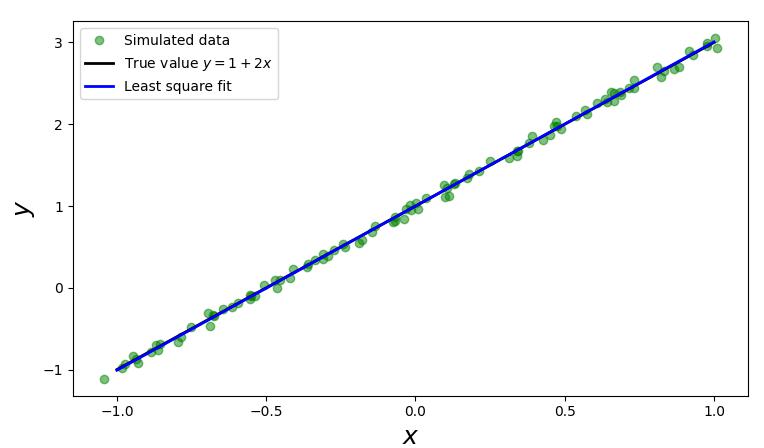
假设真实的模型是 $y=2x+1$，我们有一组数据 $(x_i,y_i)$ 共 100 个，看能否基于这 100 个数据找出 $x_i$
和 $ y_{i} $ 的线性关系方程 $ y=2 x+1 $ ，我们可以通过以下几步来完成。

1. 序构造出100个 $(x_i,y_i)$ 数据。

1
2

xi = x + np.random.normal(0, 0.05, 100)
yi = 1 + 2 * xi + np.random.normal(0, 0.05, 100)

2. 给出模型 $ f(x)=a+b x $ 的矩阵A。由于有100个观测 $ \left(x_{i}, y_{i}\right) $ 的数据，那么就有:

$$ \begin{aligned} a+b x_{0} & =y_{0} \\ a+b x_{1} & =y_{1} \\ a+b x_{2} & =y_{2} \\ \cdots & \\ a+b x_{99} & =y_{99}\end{aligned} $$

将以上式子写成如下矩阵的形式：

$$ \left|\begin{array}{cc}1 & x_{0} \\ 1 & x_{1} \\ \vdots & \vdots \\ 1 & x_{99}\end{array}\right| \times\left|\begin{array}{l}a \\ b\end{array}\right|=\left|\begin{array}{c}y_{0} \\ y_{1} \\ \vdots \\ y_{99}\end{array}\right| $$

1

A = np.vstack([xi**0, xi**1])

3. 调用 scipy.linalg.lstsq 传入 $ A^{T} $ 和观测值里的 $ y_{i} $ 即程序里的yi变量即可求得 $ f(x)=a+b x $ 里的 $a$ 和 $b$。$a$ 和 $b$ 记录在 $Istsq$ 函数的第一个返回值里。

1

sol, r, rank, s = la.lstsq(A.T, yi)

4. scipy.linalg.Istsq 的第一个返回值 sol 共有两个值， sol[0] 即是估计出来的 $ f(x)=a+b x $ 里的 $a$， $ \operatorname{sol}[1] $ 代表 $ f(x)=a+b x $ 里的 $b$。因此 $ f(x) $ 为:

1

y_fit = sol[0] + sol[1] * x 

• 示例代码

  1 2 3 4 5 6 7 8 9 10 11 12 13 14 15 16 17 18 19 20 21 22 23

  import numpy import scipy.linalg as la import numpy as np import matplotlib.pyplot as plt m = 100 x = np.linspace(-1, 1, m) y_exact = 1 + 2 * x xi = x + np.random.normal(0, 0.05, 100) yi = 1 + 2 * xi + np.random.normal(0, 0.05, 100) print (xi,"#xi") print (yi,"#yi") A = np.vstack([xi**0, xi**1]) sol, r, rank, s = la.lstsq(A.T, yi) y_fit = sol[0] + sol[1] * x print (sol,r ,rank,s ) fig, ax = plt.subplots(figsize=(12, 4)) ax.plot(xi, yi, 'go', alpha=0.5, label='Simulated data') ax.plot(x, y_exact, 'k', lw=2, label='True value $y = 1 + 2x$') ax.plot(x, y_fit, 'b', lw=2, label='Least square fit') ax.set_xlabel(r"$x$", fontsize=18) ax.set_ylabel(r"$y$", fontsize=18) ax.legend(loc=2) plt.show()

例二

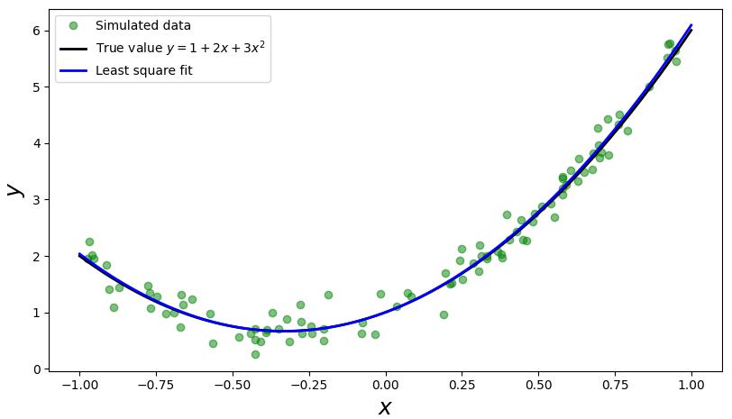
考虑模型为 $f\left(x_{i}\right)=a+b x+c x^{2} $ 的情况：

• 示例代码

  1 2 3 4 5 6 7 8 9 10 11 12 13 14 15 16 17 18 19 20 21 22 23

  import numpy import scipy.linalg as la import numpy as np import matplotlib.pyplot as plt x = np.linspace(-1, 1, 100) a, b, c = 1, 2, 3 y_exact = a + b * x + c * x**2 m = 100 xi=1 - 2 * np.random.rand(m) print ("xi.shape", xi.shape,xi**1,xi) yi=a + b * xi + c * xi**2 + np.random.randn(m) * 0.2 A = np.vstack([xi**0, xi**1, xi**2]) print (A.shape, A.T.shape) sol, r, rank, s = la.lstsq(A.T, yi) y_fit = sol[0] + sol[1] * x + sol[2] * x**2 fig, ax = plt.subplots(figsize=(12, 4)) ax.plot(xi, yi, 'go', alpha=0.5, label='Simulated data') ax.plot(x, y_exact, 'k', lw=2, label='True value $y = 1 + 2x + 3x^2$') ax.plot(x, y_fit, 'b', lw=2, label='Least square fit') ax.set_xlabel(r"$x$", fontsize=18) ax.set_ylabel(r"$y$", fontsize=18) ax.legend(loc=2) plt.show()

scipy.optimize.leastsq

• 官方文档

scipy.optimize.leastsq 方法相比于 scipy.linalg.lstsq 更加灵活，开放了 $f(x_i)$ 的模型形式。

leastsq() 函数传入误差计算函数和初始值，该初始值将作为误差计算函数的第一个参数传入。计算的结果是一个包含两个元素的元组，第一个元素是一个数组，表示拟合后的参数；第二个元素如果等于1、2、3、4中的其中一个整数，则拟合成功，否则将会返回 mesg。

调用示例

例一

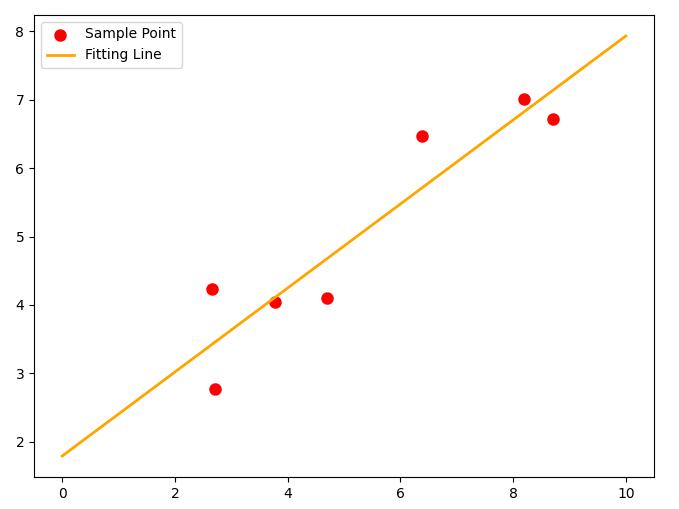
首先仍以线性拟合为例，拟合 $ f(x)=a x+b $ 函数。

• 示例代码

1
2
3
4
5
6
7
8
9
10
11
12
13
14
15
16
17
18

import numpy as np
from scipy.optimize import leastsq
def err(p, x, y):
    return p[0] * x + p[1] - y
p0 = [100, 20]
Xi=np.array([8.19,2.72,6.39,8.71,4.7,2.66,3.78])
Yi=np.array([7.01,2.78,6.47,6.71,4.1,4.23,4.05])
ret = leastsq(err, p0, args = (Xi, Yi))
print ret 
import matplotlib.pyplot as plt
k, b = ret[0]
plt.figure(figsize=(8,6))
plt.scatter(Xi,Yi,color="red",label="Sample Point",linewidth=3)
x = np.linspace(0,10,1000)
y = k * x + b
plt.plot(x,y,color="orange",label="Fitting Line",linewidth=2)
plt.legend()
plt.show()  

例二

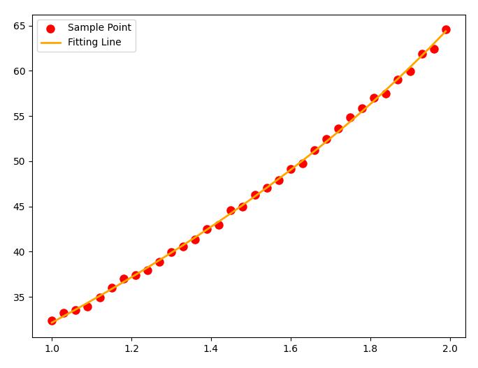
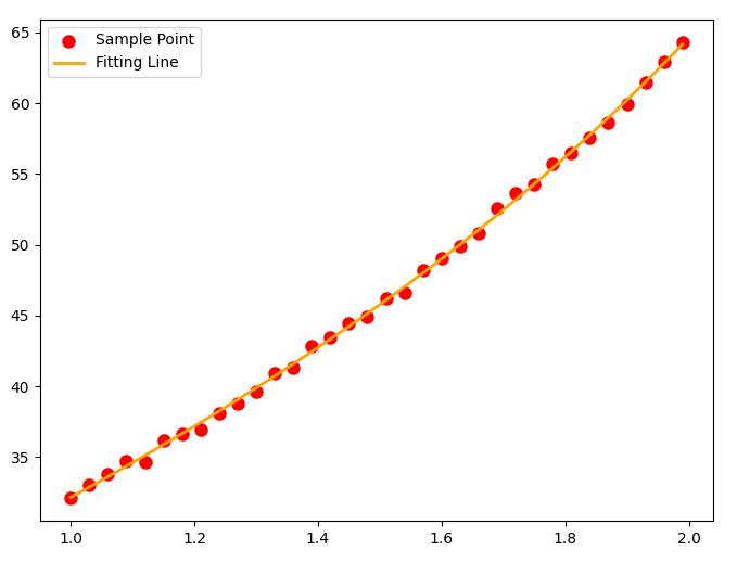
这里我们展现一下 leastsq 的灵活之处，由于 leastsq 放开了对 $f(x_i)$ 形式的严格限制，我们可以设置一些更加复杂的最小二乘的情况。

例如我现在就要拟合这么个函数：
$$
f(x)=7e^x+3\frac{1}{\sqrt{x}}+12\sin x
$$
相比于之前的多项式函数可以说有些丧心病狂了，但是也是在 leastsq 射程范围内：

1
2
3
4
5
6
7
8
9
10
11
12
13
14
15
16
17
18
19
20
21
22
23
24
25
26
27
28

import numpy as np
from scipy.optimize import leastsq
def f(p, x):
    return p[0] * (np.e ** x) + p[1] * (x ** - 0.5) + p[2] * np.sin(x)
def err(p, x, y):
    return f(p, x) - y
p0 = [1, 1, 1]
Xi = np.arange(1, 2, 0.03)
gt_p = [7, 3, 12]
Yi = f(gt_p, Xi) + (np.random.rand(len(Xi)) - 0.5)
ret = leastsq(err, p0, args = (Xi, Yi))
print (ret )
import matplotlib.pyplot as plt
plt.figure(figsize=(8,6))
plt.scatter(Xi,Yi,color="red",label="Sample Point",linewidth=3)
y = f(ret[0], Xi)
plt.plot(Xi,y,color="orange",label="Fitting Line",linewidth=2)
plt.legend()
plt.show()  

核心函数：

1

ret = leastsq(err, p0, args = (Xi, Yi))

• 其中: err 为用于计算残差的 Callback 函数，p0 为初始解， args 为输入的数据。

输出结果：

1

array([ 7.02880266,  3.16343491, 11.73254754]), 1)

优化方法不是万能的，如果矩阵过于奇异，也是不利于准确求解模型参数的。

scipy.optimize.curve_fit

• 官方文档

scipy.optimize.curve_fit 函数用于拟合曲线，给出模型和数据就可以拟合，相比于 leastsq 来说使用起来方便的地方在于不需要输入初始值。

1

scipy.optimize.curve_fit(fun, X, Y)

其中 fun 为输入参数为 $x$ 和模型参数列表，输出 $y$ 的 Callback 函数，$X$ 和 $Y$ 为数据

调用示例

例一

为了方便对比，将上文例二的示例代码修改成 curve_fit 函数的实现

• 示例代码：

1
2
3
4
5
6
7
8
9
10
11
12
13
14
15
16
17
18
19
20
21
22
23
24

import numpy as np
from scipy.optimize import curve_fit
def f(x, p0, p1, p2):
    return p0 * (np.e ** x) + p1 * (x ** - 0.5) + p2 * np.sin(x)
Xi = np.arange(1, 2, 0.03)
gt_p = [7, 3, 12]
Yi = f(Xi, *gt_p) + (np.random.rand(len(Xi)) - 0.5)
para, pcov = curve_fit(f, Xi, Yi)
print (para)
import matplotlib.pyplot as plt
plt.figure(figsize=(8,6))
plt.scatter(Xi,Yi,color="red",label="Sample Point",linewidth=3)
y = f(Xi, *(para.tolist()))
plt.plot(Xi,y,color="orange",label="Fitting Line",linewidth=2)
plt.legend()
plt.show()  

输出结果：

1

[ 6.96284945  3.03529598 12.11638088]

绘制图像：

效果没有 leastsq 稳定，可能是没有初始值的缘故。

参考资料

• http://liao.cpython.org/scipy07.html
• https://docs.scipy.org/doc/scipy/reference/generated/scipy.linalg.lstsq.html#scipy.linalg.lstsq
• https://docs.scipy.org/doc/scipy/reference/generated/scipy.optimize.leastsq.html
• https://docs.scipy.org/doc/scipy/reference/generated/scipy.optimize.curve_fit.html#scipy.optimize.curve_fit
• http://liao.cpython.org/scipytutorial07.html#7-scipy-tutorial-
• https://zhuanlan.zhihu.com/p/72241280
• https://huhuhang.com/post/machine-learning/scipy-optimize-leastsq
• https://hg95.github.io/numpy-pandas-scipy/Chapter3/拟合与优化optimize/最小二乘法拟合leastsq.html
• https://blog.csdn.net/sunbright/article/details/24717963
• http://python.circuitpython.cn/scipy05/index.html

文章链接：
https://www.zywvvd.com/notes/coding/python/scipy-leastsquare/scipy-leastsquare/