路径插值是将离散的路径点（waypoints）转换为平滑连续曲线的过程，是机器人轨迹规划、自动驾驶、CNC加工等领域的核心技术。本文深度对比五种主流插值方法：三次多项式、五次多项式、贝塞尔曲线、B样条和Clothoid回旋曲线，从数学原理、连续性分析、曲率特性和计算复杂度等多维度进行系统性研究。

问题定义与背景

什么是路径插值？

在实际应用中，路径规划通常分两步进行：

1. 全局规划：生成一系列离散的路径点（waypoints），这些点可能是障碍物避让后的转折点
2. 局部插值：在相邻路径点之间生成平滑的连续曲线，供执行机构跟踪

路径插值的核心目标：

• 曲线必须经过所有路径点（或足够接近）
• 曲线要足够平滑，避免执行机构抖动
• 曲率不能超过执行机构的物理限制（如最小转弯半径）

连续性的层级

曲线的平滑程度用连续性来度量：

曲率的物理意义

曲率 $\kappa$ 描述曲线的弯曲程度：

$$ \kappa = \frac{|x'y'' - y'x''|}{(x'^2 + y'^2)^{3/2}} $$

对于车辆：

• $\kappa = 1/R$，$R$ 是转弯半径
• $\kappa_{\max}$ 受最小转弯半径限制
• $\dot{\kappa}$（曲率变化率）与方向盘转动速度相关

1. 三次多项式插值（Cubic Polynomial）

1.1 基本原理

三次多项式是最低阶的能保证 $C^1$ 连续的多项式插值方法。最常用的形式是 Hermite 插值。

给定两个相邻路径点 $\mathbf{p}_0 = (x_0, y_0)$ 和 $\mathbf{p}_1 = (x_1, y_1)$，以及对应的切向量 $\mathbf{m}_0$ 和 $\mathbf{m}_1$，三次 Hermite 插值为：

$$ \mathbf{p}(t) = h_{00}(t) \mathbf{p}_0 + h_{10}(t) \mathbf{m}_0 + h_{01}(t) \mathbf{p}_1 + h_{11}(t) \mathbf{m}_1 $$

其中 $t \in [0,1]$ 是归一化参数，Hermite 基函数为：

$$ \begin{aligned} h_{00}(t) &= 2t^3 - 3t^2 + 1 \\ h_{10}(t) &= t^3 - 2t^2 + t \\ h_{01}(t) &= -2t^3 + 3t^2 \\ h_{11}(t) &= t^3 - t^2 \end{aligned} $$

1.2 边界条件验证

验证基函数的正确性：

在 $t=0$ 处：

$$ \begin{aligned} h_{00}(0) &= 1, \quad h_{10}(0) = 0, \quad h_{01}(0) = 0, \quad h_{11}(0) = 0 \\ \Rightarrow \mathbf{p}(0) &= \mathbf{p}_0 \quad \checkmark \end{aligned} $$

在 $t=1$ 处：

$$ \begin{aligned} h_{00}(1) &= 0, \quad h_{10}(1) = 0, \quad h_{01}(1) = 1, \quad h_{11}(1) = 0 \\ \Rightarrow \mathbf{p}(1) &= \mathbf{p}_1 \quad \checkmark \end{aligned} $$

导数：

$$ \begin{aligned} h_{00}'(t) &= 6t^2 - 6t, \quad h_{10}'(t) = 3t^2 - 4t + 1 \\ h_{00}'(0) &= 0, \quad h_{10}'(0) = 1 \\ \Rightarrow \mathbf{p}'(0) &= \mathbf{m}_0 \quad \checkmark \end{aligned} $$

1.3 切向量的估计

切向量 $\mathbf{m}$ 决定了曲线的形状，常用的估计方法：

1. Catmull-Rom 方法（推荐）：

$$ \mathbf{m}_i = \frac{\mathbf{p}_{i+1} - \mathbf{p}_{i-1}}{2} $$

2. 有限差分：

$$ \mathbf{m}_i = \frac{\mathbf{p}_{i+1} - \mathbf{p}_i}{2} $$

3. 手动指定：根据运动学约束确定

1.4 连续性分析

1.5 Python 实现

1
2
3
4
5
6
7
8
9
10
11
12
13
14
15
16
17
18
19
20
21
22
23
24
25
26
27
28
29
30
31
32
33
34
35

def cubic_hermite_interpolate(points, num_points=200):
    """Cubic Hermite Interpolation"""
    points = np.array(points)
    n = len(points)
    all_x, all_y = [], []
        for i in range(n - 1):
        p0, p1 = points[i], points[i + 1]
                # Catmull-Rom tangent estimation
        if i == 0:
            m0 = (p1 - p0) * 0.5
        else:
            m0 = (points[i+1] - points[i-1]) * 0.25
                if i == n - 2:
            m1 = (p1 - p0) * 0.5
        else:
            m1 = (points[i+2] - points[i]) * 0.25
                t = np.linspace(0, 1, num_points // (n-1) + 1)[:-1]
                # Hermite basis functions
        h00 = 2*t**3 - 3*t**2 + 1
        h10 = t**3 - 2*t**2 + t
        h01 = -2*t**3 + 3*t**2
        h11 = t**3 - t**2
                x = h00*p0[0] + h10*m0[0] + h01*p1[0] + h11*m1[0]
        y = h00*p0[1] + h10*m0[1] + h01*p1[1] + h11*m1[1]
                all_x.extend(x)
        all_y.extend(y)
        return np.array(all_x), np.array(all_y)

1.6 优缺点总结

优点：

• 计算简单，效率高
• 可以精确控制端点速度
• $C^2$ 连续性满足大多数应用需求

缺点：

• 加加速度不连续，高速时可能引起振动
• 无法保证曲率连续
• 对切向量估计敏感，可能产生过冲

2. 五次多项式插值（Quintic Polynomial）

2.1 为什么需要五次多项式？

三次多项式的加速度是线性函数，加加速度（jerk）是常数。在段连接处，加加速度会突变，导致高频振动。

五次多项式有6个自由度，可以满足6个边界条件，实现 $C^3$ 连续。

2.2 数学形式

$$ \mathbf{p}(t) = \mathbf{a}_0 + \mathbf{a}_1 t + \mathbf{a}_2 t^2 + \mathbf{a}_3 t^3 + \mathbf{a}_4 t^4 + \mathbf{a}_5 t^5 $$

边界条件（6个方程）：

$$ \begin{aligned} \mathbf{p}(0) &= \mathbf{p}_0, \quad \mathbf{p}(1) = \mathbf{p}_1 \\ \mathbf{p}'(0) &= \mathbf{v}_0, \quad \mathbf{p}'(1) = \mathbf{v}_1 \\ \mathbf{p}''(0) &= \mathbf{a}_0, \quad \mathbf{p}''(1) = \mathbf{a}_1 \end{aligned} $$

2.3 系数求解

写成矩阵形式 $\mathbf{A}\mathbf{c} = \mathbf{b}$：

$$ \begin{bmatrix} 1 & 0 & 0 & 0 & 0 & 0 \\ 0 & 1 & 0 & 0 & 0 & 0 \\ 0 & 0 & 2 & 0 & 0 & 0 \\ 1 & 1 & 1 & 1 & 1 & 1 \\ 0 & 1 & 2 & 3 & 4 & 5 \\ 0 & 0 & 2 & 6 & 12 & 20 \end{bmatrix} \begin{bmatrix} a_0 \\ a_1 \\ a_2 \\ a_3 \\ a_4 \\ a_5 \end{bmatrix} = \begin{bmatrix} p_0 \\ v_0 \\ a_0 \\ p_1 \\ v_1 \\ a_1 \end{bmatrix} $$

2.4 Python 实现

1
2
3
4
5
6
7
8
9
10
11
12
13
14
15
16
17
18
19
20
21
22
23
24
25
26
27
28
29
30
31
32
33
34
35
36
37
38
39
40

def quintic_polynomial_interpolate(points, num_points=200):
    """Quintic Polynomial Interpolation with C3 continuity"""
    points = np.array(points)
    n = len(points)
    all_x, all_y = [], []
        for i in range(n - 1):
        p0, p1 = points[i], points[i + 1]
                # Estimate velocity and acceleration
        v0 = (points[i+1] - points[max(0, i-1)]) * 0.15
        v1 = (points[min(n-1, i+2)] - points[max(0, i-1)]) * 0.15
        a0, a1 = np.zeros(2), np.zeros(2)  # Zero acceleration at endpoints
                # Solve for coefficients
        def solve_coeffs(p0, p1, v0, v1, a0, a1):
            A = np.array([
                [1, 0, 0, 0, 0, 0],
                [0, 1, 0, 0, 0, 0],
                [0, 0, 2, 0, 0, 0],
                [1, 1, 1, 1, 1, 1],
                [0, 1, 2, 3, 4, 5],
                [0, 0, 2, 6, 12, 20]
            ])
            b = np.array([p0, v0, a0, p1, v1, a1])
            return np.linalg.solve(A, b)
                coeffs_x = solve_coeffs(p0[0], p1[0], v0[0], v1[0], a0[0], a1[0])
        coeffs_y = solve_coeffs(p0[1], p1[1], v0[1], v1[1], a0[1], a1[1])
                t = np.linspace(0, 1, num_points // (n-1) + 1)[:-1]
        t_powers = np.vstack([t**i for i in range(6)])
                x = coeffs_x @ t_powers
        y = coeffs_y @ t_powers
                all_x.extend(x)
        all_y.extend(y)
        return np.array(all_x), np.array(all_y)

2.5 优缺点总结

优点：

• $C^3$ 连续性，加加速度平滑
• 可以精确控制端点加速度
• 运动更加舒适，振动小

缺点：

• 计算复杂度更高
• 可能产生更大的过冲
• 曲率仍不连续

3. 贝塞尔曲线（Bézier Curve）

3.1 数学定义

n次贝塞尔曲线定义为：

$$ \mathbf{B}(t) = \sum_{i=0}^{n} B_{i,n}(t) \mathbf{P}_i, \quad t \in [0,1] $$

其中 $\mathbf{P}i$ 是控制点，$B{i,n}(t)$ 是伯恩斯坦基函数：

$$ B_{i,n}(t) = \binom{n}{i} (1-t)^{n-i} t^i = \frac{n!}{i!(n-i)!} (1-t)^{n-i} t^i $$

3.2 三次贝塞尔曲线

三次贝塞尔（$n=3$）是最常用的形式：

$$ \mathbf{B}(t) = (1-t)^3\mathbf{P}_0 + 3(1-t)^2t\mathbf{P}_1 + 3(1-t)t^2\mathbf{P}_2 + t^3\mathbf{P}_3 $$

展开基函数：

$$ \begin{aligned} B_{0,3}(t) &= (1-t)^3 \\ B_{1,3}(t) &= 3(1-t)^2t \\ B_{2,3}(t) &= 3(1-t)t^2 \\ B_{3,3}(t) &= t^3 \end{aligned} $$

3.3 重要性质

3.4 de Casteljau 算法

递归计算贝塞尔曲线点的稳定算法：

$$ \mathbf{P}_i^{(k)} = (1-t)\mathbf{P}_i^{(k-1)} + t\mathbf{P}_{i+1}^{(k-1)} $$

其中 $\mathbf{P}_i^{(0)} = \mathbf{P}_i$，最终 $\mathbf{B}(t) = \mathbf{P}_0^{(n)}$。

3.5 从路径点到控制点

贝塞尔曲线不通过中间控制点。要使曲线通过给定路径点，需要反算控制点。

常用方法：Catmull-Rom 到贝塞尔转换

给定 Catmull-Rom 样条的控制点 $\mathbf{P}_0, \mathbf{P}_1, \mathbf{P}_2, \mathbf{P}_3$，等价的贝塞尔控制点为：

$$ \begin{aligned} \mathbf{B}_0 &= \mathbf{P}_1 \\ \mathbf{B}_1 &= \mathbf{P}_1 + \frac{\mathbf{P}_2 - \mathbf{P}_0}{6} \\ \mathbf{B}_2 &= \mathbf{P}_2 - \frac{\mathbf{P}_3 - \mathbf{P}_1}{6} \\ \mathbf{B}_3 &= \mathbf{P}_2 \end{aligned} $$

3.6 Python 实现

1
2
3
4
5
6
7
8
9
10
11
12
13
14
15
16
17
18
19
20
21
22
23
24
25
26
27
28
29
30
31
32
33

def bezier_interpolate(points, num_points=200):
    """Cubic Bezier Curve with Catmull-Rom to Bezier conversion"""
    points = np.array(points)
    n = len(points)
    all_x, all_y = [], []
        for i in range(n - 1):
        p0 = points[max(0, i-1)]
        p1 = points[i]
        p2 = points[i+1]
        p3 = points[min(n-1, i+2)]
                # Catmull-Rom to Bezier control points
        cp1 = p1 + (p2 - p0) / 6
        cp2 = p2 - (p3 - p1) / 6
                ctrl_pts = np.array([p1, cp1, cp2, p2])
                t = np.linspace(0, 1, num_points // (n-1) + 1)[:-1]
                # Bernstein basis functions
        b0 = (1-t)**3
        b1 = 3*(1-t)**2*t
        b2 = 3*(1-t)*t**2
        b3 = t**3
                x = b0*ctrl_pts[0,0] + b1*ctrl_pts[1,0] + b2*ctrl_pts[2,0] + b3*ctrl_pts[3,0]
        y = b0*ctrl_pts[0,1] + b1*ctrl_pts[1,1] + b2*ctrl_pts[2,1] + b3*ctrl_pts[3,1]
                all_x.extend(x)
        all_y.extend(y)
        return np.array(all_x), np.array(all_y)

3.7 优缺点总结

优点：

• 几何性质优良，凸包保证曲线可控
• 控制点直观，便于交互设计
• de Casteljau 算法数值稳定

缺点：

• 缺乏局部控制性（移动控制点影响整条曲线）
• 单段曲线无法通过多个给定点
• 段间 $C^2$ 连续性需要额外约束

4. B样条曲线（B-Spline）

4.1 为什么需要B样条？

贝塞尔曲线的主要问题是缺乏局部控制性——移动一个控制点会影响整条曲线。B样条通过引入基函数的局部支撑性解决了这个问题。

4.2 数学定义

B样条曲线定义为：

$$ \mathbf{C}(u) = \sum_{i=0}^{n} N_{i,p}(u) \mathbf{P}_i, \quad u \in [u_p, u_{m-p}] $$

其中 $N_{i,p}(u)$ 是 p次B样条基函数，$\mathbf{P}_i$ 是控制点。

4.3 Cox-de Boor 递归公式

基函数通过递归定义：

$$ \begin{aligned} N_{i,0}(u) &= \begin{cases} 1 & u_i \le u < u_{i+1} \\ 0 & \text{otherwise} \end{cases} \\[10pt] N_{i,p}(u) &= \frac{u - u_i}{u_{i+p} - u_i} N_{i,p-1}(u) + \frac{u_{i+p+1} - u}{u_{i+p+1} - u_{i+1}} N_{i+1,p-1}(u) \end{aligned} $$

节点向量 $\mathbf{U} = {u_0, u_1, \ldots, u_m}$ 决定了基函数的支撑范围。

4.4 局部支撑性

$N_{i,p}(u)$ 仅在 $[u_{i}, u_{i+p+1})$ 上非零。这意味着：

• 移动控制点 $\mathbf{P}{i}$ 只影响 $[u{i}, u_{i+p+1})$ 区间的曲线
• 曲线的局部修改不会影响其他部分

4.5 连续性

在非重复节点处，p次B样条具有 $C^{p-1}$ 连续性：

4.6 节点向量类型

1. 均匀节点：

$$ u_i = \frac{i}{m}, \quad i = 0, 1, \ldots, m $$

2. 弦长参数化（推荐）：

$$ u_i = \frac{\sum_{j=1}^{i} \|\mathbf{P}_j - \mathbf{P}_{j-1}\|}{\sum_{j=1}^{n} \|\mathbf{P}_j - \mathbf{P}_{j-1}\|} $$

3. 向心参数化：

$$ u_i = \frac{\sum_{j=1}^{i} \sqrt{\|\mathbf{P}_j - \mathbf{P}_{j-1}\|}}{\sum_{j=1}^{n} \sqrt{\|\mathbf{P}_j - \mathbf{P}_{j-1}\|}} $$

4.7 Python 实现

1
2
3
4
5
6
7
8
9
10
11
12
13
14

from scipy.interpolate import splprep, splev
def bspline_interpolate(points, degree=3, num_points=200):
    """B-Spline Curve using scipy"""
    points = np.array(points)
        # s=0 means interpolation (pass through all points)
    # k is the spline degree
    tck, u = splprep([points[:, 0], points[:, 1]], s=0, k=degree)
        u_new = np.linspace(0, 1, num_points)
    x_new, y_new = splev(u_new, tck)
        return np.array(x_new), np.array(y_new)

4.8 优缺点总结

优点：

• 局部控制性：修改局部不影响其他部分
• 高阶连续性（取决于次数）
• 变差缩减性质
• 包含贝塞尔曲线作为特例

缺点：

• 不通过中间控制点（除非使用插值B样条）
• 参数化对曲线形状有影响
• 概念相对复杂

5. Clothoid（回旋曲线/Euler Spiral）

5.1 什么是Clothoid？

Clothoid曲线（也称回旋曲线、Cornu螺线或Euler螺线）的核心特性是曲率随弧长线性变化：

$$ \kappa(s) = \kappa_0 + c \cdot s $$

其中 $\kappa_0$ 是起始曲率，$c$ 是曲率变化率（sharpness），$s$ 是弧长参数。

5.2 几何推导

切向角随弧长的变化：

$$ \theta(s) = \theta_0 + \int_0^s \kappa(t) \, dt = \theta_0 + \kappa_0 s + \frac{c s^2}{2} $$

参数方程：

$$ \begin{aligned} x(s) &= x_0 + \int_0^s \cos\theta(t) \, dt = x_0 + \int_0^s \cos\left(\theta_0 + \kappa_0 t + \frac{c t^2}{2}\right) dt \\ y(s) &= y_0 + \int_0^s \sin\theta(t) \, dt = y_0 + \int_0^s \sin\left(\theta_0 + \kappa_0 t + \frac{c t^2}{2}\right) dt \end{aligned} $$

这被称为Fresnel积分。

5.3 物理意义

Clothoid 是唯一满足曲率连续且线性变化的曲线，这使得它：

1. 符合人类驾驶行为：驾驶员以恒定角速度转动方向盘，行驶轨迹就是Clothoid
2. 舒适性最优：曲率线性变化意味着横向加速度线性变化，加加速度最小
3. 被广泛应用于道路设计：连接直线和圆弧的过渡曲线

5.4 特殊情况

5.5 Python 实现

1
2
3
4
5
6
7
8
9
10
11
12
13
14
15
16
17
18
19
20
21
22
23
24
25
26
27
28
29
30
31
32
33
34
35
36
37
38
39
40
41
42
43
44
45

from scipy.integrate import quad
def clothoid_fresnel(s, theta0, kappa0, c):
    """Clothoid Fresnel Integrals"""
    def integrand_x(t):
        theta = theta0 + kappa0 * t + 0.5 * c * t**2
        return np.cos(theta)
        def integrand_y(t):
        theta = theta0 + kappa0 * t + 0.5 * c * t**2
        return np.sin(theta)
        x, _ = quad(integrand_x, 0, s, limit=100)
    y, _ = quad(integrand_y, 0, s, limit=100)
        return x, y
def clothoid_interpolate(points, num_points=200):
    """Clothoid Interpolation"""
    points = np.array(points)
    n = len(points)
    all_x, all_y = [], []
        for i in range(n - 1):
        p0, p1 = points[i], points[i + 1]
                # Calculate tangent angles
        theta0 = np.arctan2(p1[1] - p0[1], p1[0] - p0[0])
        length = np.linalg.norm(p1 - p0)
                # Clothoid parameters
        kappa0 = 0  # Starting curvature
        c = 0  # Curvature rate (simplified)
                s_values = np.linspace(0, length, num_points // (n-1) + 1)[:-1]
                for s in s_values:
            dx, dy = clothoid_fresnel(s, theta0, kappa0, c)
            # Transform to global coordinates
            x = dx * np.cos(theta0) - dy * np.sin(theta0) + p0[0]
            y = dx * np.sin(theta0) + dy * np.cos(theta0) + p0[1]
            all_x.append(x)
            all_y.append(y)
        return np.array(all_x), np.array(all_y)

5.6 优缺点总结

优点：

• 曲率连续：最适合道路和铁路设计
• 舒适性最优：符合人类驾驶行为
• 最小化加加速度

缺点：

• 计算复杂（需要数值积分）
• 无法精确通过任意给定点
• 参数求解是非线性问题

6. 实验对比

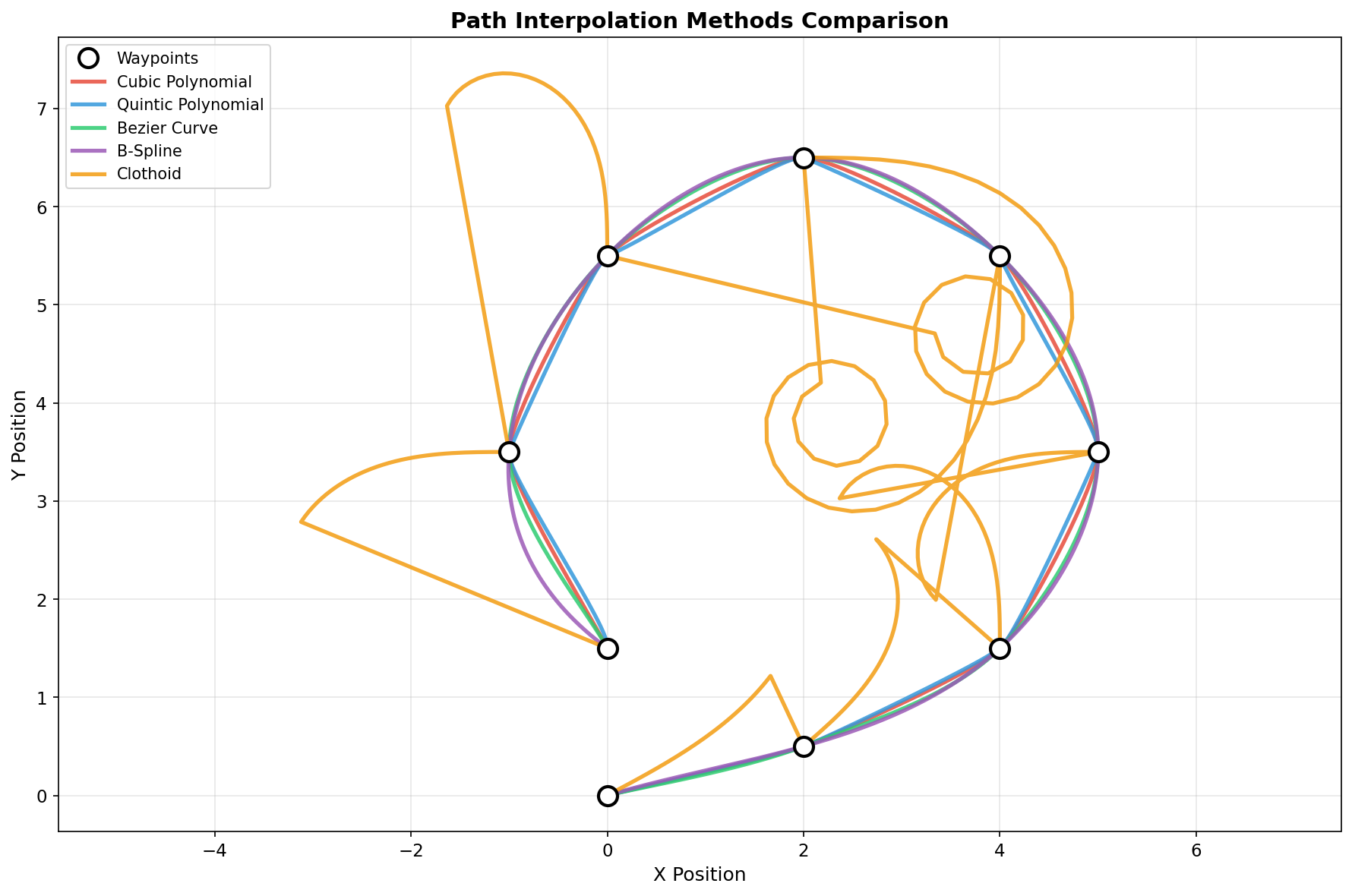
6.1 测试路径说明

我们使用 9 个路径点构成的测试路径，模拟一个典型的机器人或车辆行驶场景：

1
2
3
4
5
6
7
8
9
10
11

waypoints = np.array([
    [0, 0],      # 起点
    [2, 0.5],    # 第一转弯
    [4, 1.5],    # 
    [5, 3.5],    # 顶点
    [4, 5.5],    # 
    [2, 6.5],    # 
    [0, 5.5],    # 
    [-1, 3.5],   # 最后转弯
    [0, 1.5]     # 终点（接近起点，形成闭环）
])

这个路径包含：

• 直线段
• 缓弯
• 急转弯
• S形弯道

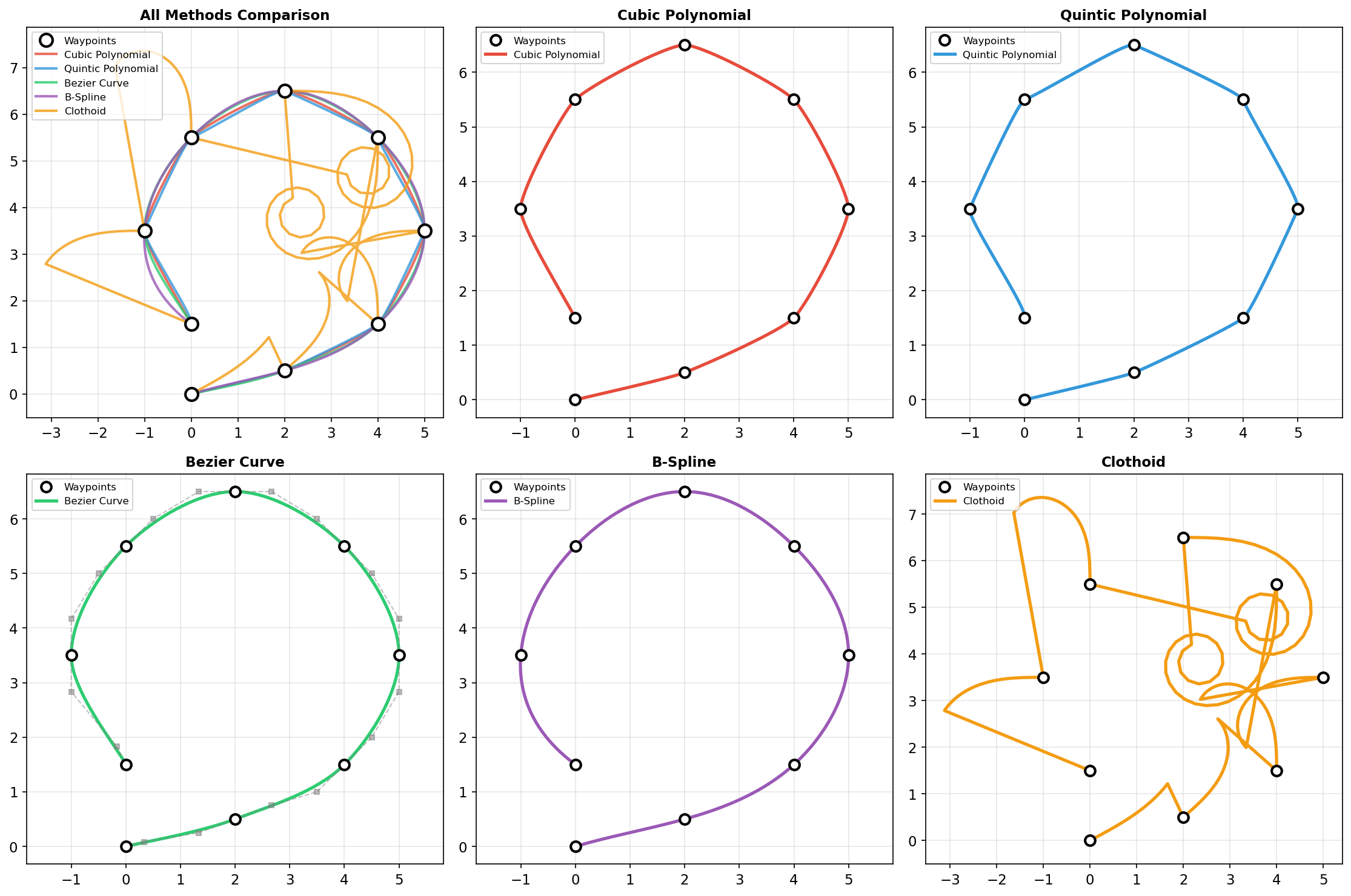
6.2 路径对比

观察要点：

• 所有方法都经过路径点（或接近路径点）
• 贝塞尔和B样条曲线更加平滑
• Clothoid在某些情况下可能偏离路径点

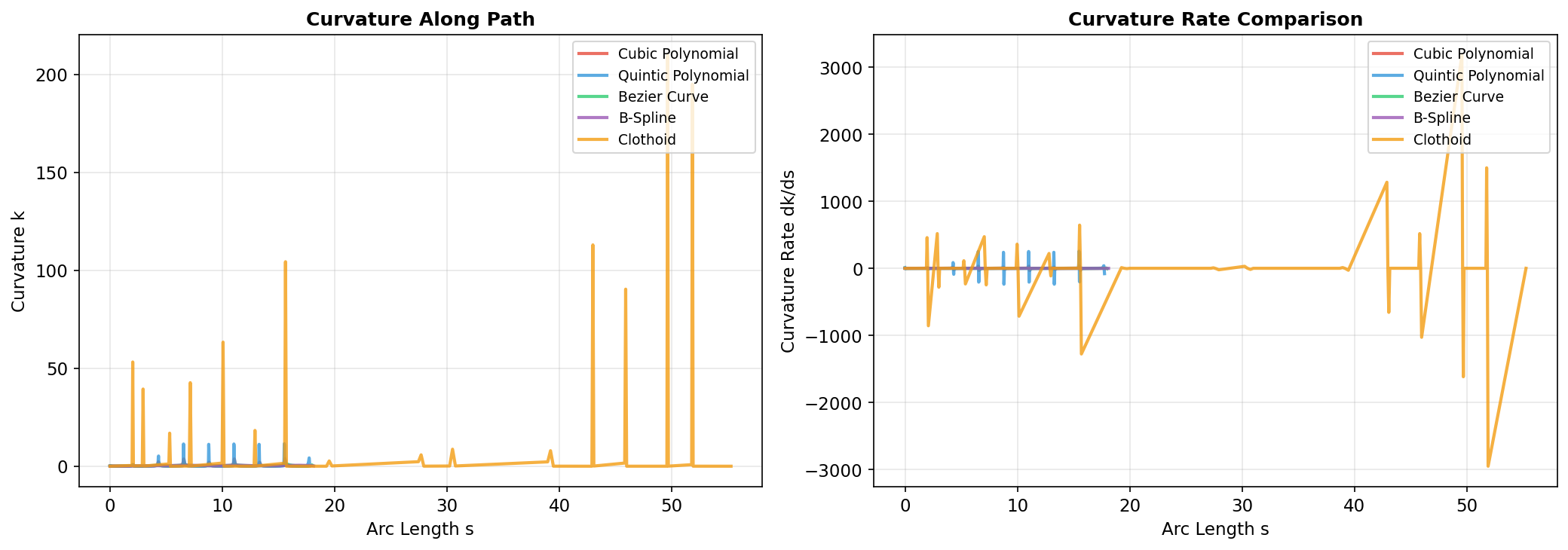
6.3 曲率分析

曲率是衡量曲线弯曲程度的关键指标：

$$ \kappa = \frac{|x'y'' - y'x''|}{(x'^2 + y'^2)^{3/2}} $$

曲率变化率（与加加速度/舒适性相关）：

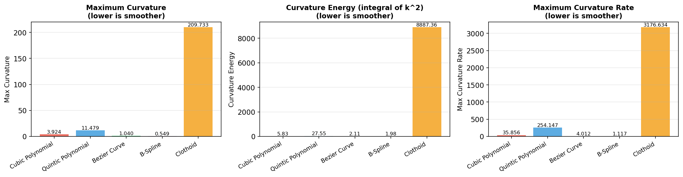
6.4 量化指标

指标解释：

• 最大曲率：越小越好，受最小转弯半径限制
• 曲率能量：越小越平滑
• 最大曲率变化率：越小越舒适

6.5 各方法详细对比

7. 深度分析与选择指南

7.1 连续性对比

1
2
3
4
5
6
7
8
9
10
11
12
13
14

C^0 ──────────────────────────────────────────► 所有方法
     位置连续
         
C^1 ──────────────────────────────────────────► 所有方法
     速度连续
         
C^2 ──────────────────────────────────────────► 所有方法
     加速度连续
         
C^3 ──────────────────────────────────────────► 五次多项式、B样条(p≥4)
     加加速度连续
         
G^1 ──────────────────────────────────────────► Clothoid
     曲率连续

7.2 应用场景推荐

7.3 计算复杂度对比

7.4 关键洞察

1. 平滑度与计算成本的权衡：高连续性（如$C^3$、$G1$）需要更复杂的计算

2. 曲率是转向的关键：

   • 机器人/车辆有最大曲率限制（最小转弯半径）
   • 曲率变化率影响控制器响应

3. 没有万能的方法：

   • 根据具体应用场景选择
   • 可以组合使用（如：直线段用Clothoid连接，中间用B样条）

4. 参数化问题：

   • 弧长参数化 vs 均匀参数化
   • 参数化方式影响速度规划

8. 完整代码

1
2
3
4
5
6
7
8
9
10
11
12
13
14
15
16
17
18
19
20
21
22
23
24
25
26
27
28
29
30
31
32
33
34
35
36
37
38
39
40
41
42
43
44

"""
Path Interpolation Methods Comparison
Complete implementation with all five methods
"""
import numpy as np
import matplotlib.pyplot as plt
from scipy.interpolate import splprep, splev
from scipy.integrate import quad
def compute_curvature(x, y):
    """Compute curvature: k = |x'y'' - y'x''| / (x'^2 + y'^2)^(3/2)"""
    dx = np.gradient(x)
    dy = np.gradient(y)
    ddx = np.gradient(dx)
    ddy = np.gradient(dy)
        curvature = np.abs(dx * ddy - dy * ddx) / (dx**2 + dy**2)**1.5
    return np.nan_to_num(curvature, nan=0.0)
def compute_arc_length(x, y):
    """Compute arc length"""
    ds = np.sqrt(np.diff(x)**2 + np.diff(y)**2)
    return np.concatenate([[0], np.cumsum(ds)])
# Main test
if __name__ == "__main__":
    # Test waypoints
    waypoints = np.array([
        [0, 0], [2, 0.5], [4, 1.5], [5, 3.5],
        [4, 5.5], [2, 6.5], [0, 5.5], [-1, 3.5], [0, 1.5]
    ])
        # Compute all methods
    methods = {
        'Cubic': cubic_hermite_interpolate(waypoints),
        'Quintic': quintic_polynomial_interpolate(waypoints),
        'Bezier': bezier_interpolate(waypoints),
        'B-Spline': bspline_interpolate(waypoints),
        'Clothoid': clothoid_interpolate(waypoints)
    }
        # Plot comparison
    # ...

9. 总结

9.1 方法对比表

9.2 选择建议

• 追求舒适性（载人车辆、电梯）→ Clothoid 或 五次多项式
• 追求效率（工业机器人）→ 三次多项式
• 需要局部调整（交互式设计）→ B样条
• 图形/动画应用 → 贝塞尔曲线

参考资料

• [1] Farin, G. (2002). Curves and Surfaces for CAGD: A Practical Guide. Morgan Kaufmann.
• [2] Piegl, L., & Tiller, W. (1997). The NURBS Book. Springer.
• [3] Brezak, M., & Petrović, I. (2012). Real-time approximation of clothoids with bounded error for path planning applications. IEEE.
• [4] Prautzsch, H., Boehm, W., & Paluszny, M. (2002). Bézier and B-Spline Techniques. Springer.
• [5] Bertolazzi, E., & Frego, M. (2015). Interpolating clothoid splines with curvature continuity. Mathematical Methods in the Applied Sciences.

文章链接：
https://www.zywvvd.com/notes/study/algorithm/path-interpolation-comparison/path-interpolation-comparison/