This is a six-part deep-dive series on AI compute — the most important and least understood layer of modern AI systems.

While most discussions focus on models, real-world performance is determined by compute, memory, and communication constraints.

This series aims to demystify the hardware and systems behind AI.

In Part 1, we build the foundation — understanding the AI compute landscape and the evolution of system bottlenecks.

AI progress today is no longer limited by models alone.

It is constrained by the systems that run them — compute, memory, and interconnect.

Training frontier AI systems now requires thousands to tens of thousands of GPUs operating in parallel, while serving modern models at scale demands careful optimization of memory bandwidth, latency, and cost. As models grow larger and workloads become more complex, the hardware layer has evolved into a critical determinant of performance.

At the same time, the AI compute ecosystem has become increasingly fragmented. Engineers must navigate a rapidly expanding set of options — GPUs, TPUs, specialized accelerators, and distributed clusters — each with distinct strengths, limitations, and operational tradeoffs.

Despite this complexity, clear guidance on how these systems work — and when to use each — remains limited.

This raises a fundamental question:

Which hardware should we actually use for AI?

This chapter builds a foundational understanding of the AI compute landscape, introducing the hardware, system-level constraints, and architectural tradeoffs that underpin modern AI workloads.

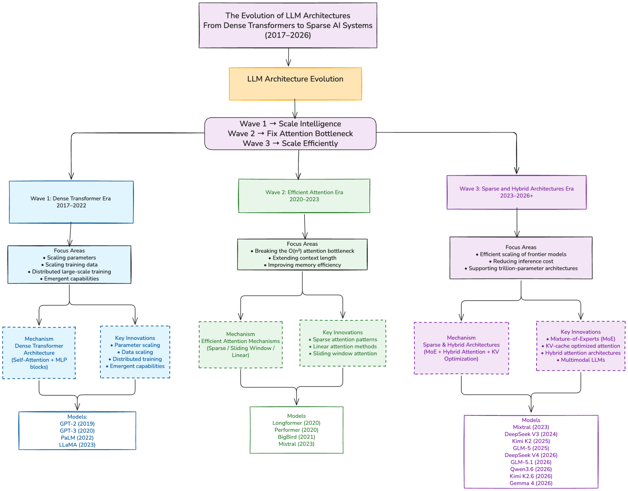
The Evolution of AI Bottlenecks

The evolution of modern AI systems is often described through changes in model architectures — from dense transformers to efficient attention and sparse systems.

However, a more fundamental way to understand this progression is through shifting system bottlenecks.

Wave 1: Compute-Bound (Scale Intelligence)(2017–2022)

The first wave of large language models focused on scaling:

• Increasing model parameters

• Expanding training data

• Distributed large-scale training

Performance improvements were primarily driven by increasing training compute, following scaling laws.

The dominant constraint in this phase was compute — more FLOPs, more GPUs, and longer training cycles.

Wave 2: Memory-Bound (Fix Attention Bottleneck)(2020–2023)

As models grew larger and context lengths increased, new limitations emerged:

• Quadratic attention complexity

• Growth in intermediate activations and KV cache

• Memory bandwidth and capacity constraints

This led to innovations such as:

• Sparse attention

• Linear attention

• Sliding window mechanisms

The bottleneck shifted from compute to memory (capacity and bandwidth).

Wave 3: System-Bound (Scale Efficiently)(2023+)

In the current wave, AI systems operate at extreme scale:

• Trillion-parameter models

• Multi-node distributed training

• High-throughput, low-latency inference

At this stage, no single resource dominates performance. Instead, systems are constrained by multiple factors simultaneously:

• Compute → large-scale training and inference

• Memory → model weights, activations, KV cache

• Interconnect → communication across GPUs and nodes

The bottleneck is now the entire system.

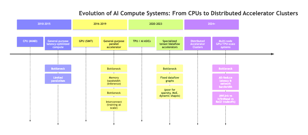
The evolution of AI compute reflects a consistent pattern: hardware architectures adapt to the dominant computational structure of AI workloads, and in doing so, shift the primary system bottleneck.

Early machine learning workloads ran on CPUs, which follow a MIMD (Multiple Instruction, Multiple Data) model. CPUs are optimized for flexibility and low-latency execution, making them well-suited for control-heavy workloads. However, they offer limited parallelism, which becomes a bottleneck for large-scale numerical computation.

Deep learning introduced a different workload profile — large, repetitive matrix operations applied across massive datasets. GPUs, built around a SIMT (Single Instruction, Multiple Threads) model, are designed for this pattern. By executing thousands of threads in parallel, GPUs deliver significantly higher throughput, making them the default platform for training neural networks.

As models continued to scale, further specialization emerged. TPUs and other AI accelerators optimize for dense tensor operations using structured dataflows and reduced-precision arithmetic. These systems trade flexibility for efficiency, targeting specific compute patterns common in large-scale training.

At the same time, the limiting factors shifted. While early GPU workloads were primarily compute-bound, modern AI systems increasingly encounter memory bandwidth constraints during inference and communication overhead during distributed training. The introduction of transformer architectures accelerated this trend, making high-bandwidth memory and fast interconnects critical for performance.

Today, AI compute operates at cluster scale. Modern workloads run on distributed accelerator systems, where performance depends not only on compute throughput, but also on interconnect bandwidth and collective communication efficiency. Scaling is no longer a device-level problem — it is a system-level problem.

Importantly, this evolution is not a sequence of replacements, but a layering of systems:

• CPUs handle orchestration and data pipelines

• GPUs perform the majority of compute

• TPUs and ASICs target specialized workloads

• Distributed clusters enable large-scale execution

From Architecture Evolution to Execution Reality

The previous diagram showed how AI compute evolved across hardware generations.
This diagram shows the same story from a different lens:

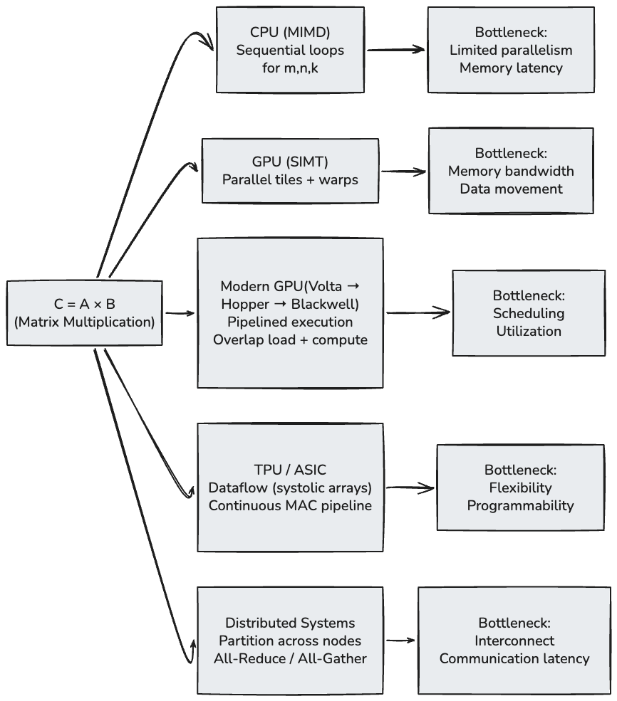
how a single operation — matrix multiplication — is executed across systems

At a high level, nothing changes:

C = A × B

But the execution model changes dramatically.

• On CPUs, the computation is performed using nested loops, processing one output element at a time with limited parallelism.

• On GPUs, the same operation is restructured into parallel tiles, allowing thousands of threads to compute multiple outputs simultaneously.

• On modern GPUs, execution is further optimized by overlapping data movement and compute, ensuring hardware units remain utilized.

• On accelerators (TPUs/ASICs), the computation is mapped into dataflow pipelines, where multiply-accumulate operations happen continuously as data flows through hardware.

• In distributed systems, the problem is partitioned across devices, and the final result is obtained through communication and aggregation.

While the computation remains identical, the system bottleneck shifts at each stage

Modern AI systems are not defined by a single component, but by a stack of tightly coupled layers — from applications down to hardware and infrastructure.

Understanding this stack is critical because:

Performance bottlenecks can originate at any layer — and propagate across the entire system.

The AI Compute Stack (End-to-End View)

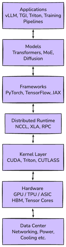
Layer-by-Layer Breakdown

1. Applications Layer

• Inference systems (vLLM, TGI, Triton)

• Training pipelines

• APIs and serving systems

Defines:

• latency requirements

• throughput targets

• cost constraints

2. Model Layer

• Transformers, MoE, Diffusion

• Determines:

  • compute intensity

  • memory footprint

  • communication pattern

Example:

• Attention → memory-heavy

• MoE → communication-heavy

3. Framework Layer

• PyTorch, TensorFlow, JAX

• Handles:

  • computation graphs

  • autograd

  • execution planning

Converts models into executable operations

4. Distributed Runtime

• NCCL, XLA, RPC systems

• Responsible for:

  • All-Reduce, All-Gather

  • synchronization

  • multi-node execution

This is where interconnect becomes critical

5. Kernel Layer

• CUDA, Triton, CUTLASS

• Implements:

  • matrix multiplication

  • attention kernels

  • fused operations

Determines actual GPU utilization

6. Hardware Layer

• GPUs, TPUs, ASICs

• Components:

  • Tensor cores

  • HBM memory

  • on-chip caches

Defines:

• FLOPs

• memory bandwidth

• parallelism

7. Data Center Layer

• Networking (InfiniBand, RoCE)

• Power, cooling, racks

Enables:

• cluster-scale AI

• distributed training and inference

So Basically a change in one layer affects all others:

• Model → memory → kernel → hardware utilization

• Hardware → kernel design → model optimization

• Network → distributed strategy → model architecture

Example: One Bottleneck Across the Stack

Problem: KV Cache Explosion in LLM Inference

• Model layer → large context → KV cache grows

• Hardware layer → HBM pressure increases

• Kernel layer → memory-bound execution

• Application layer → latency increases

One design decision cascades through the stack.

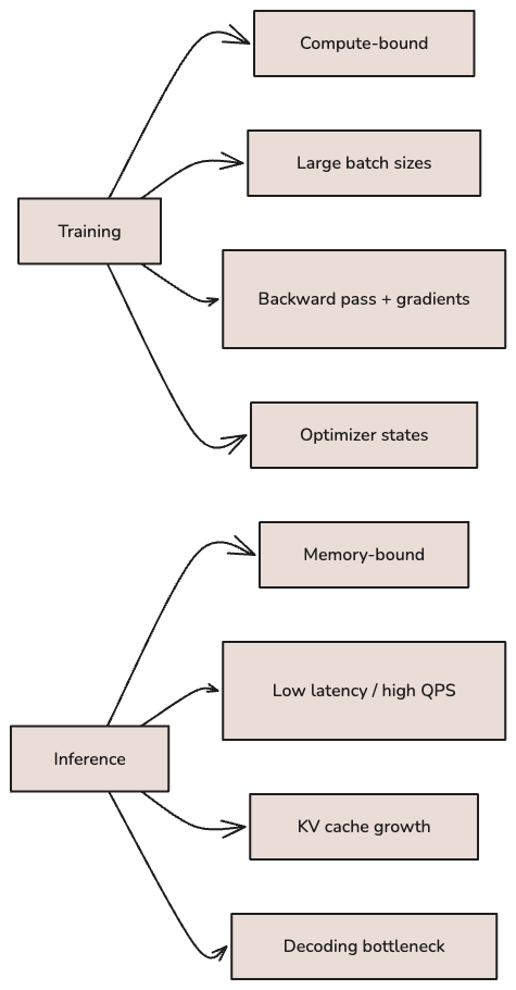
Modern AI systems operate under two fundamentally different workloads:

• Training (building the model)

• Inference (using the model)

While both rely on the same underlying computation (e.g., matrix multiplication), they place very different demands on the system.

4.1 Workload Characteristics

Training

• Dominated by forward + backward passes

• Large batch sizes

• Heavy use of:

  • gradients

  • optimizer states (Adam, etc.)

Focus: maximize throughput

Inference

• Only forward pass

• Often autoregressive (token-by-token)

• Strict latency constraints

Focus: minimize latency + cost

4.2 Compute vs Memory Behavior

Training → Compute-Bound

• Large matrix multiplications

• High arithmetic intensity

• Efficient GPU utilization

High FLOPs utilization (MFU) → critical metric

Inference → Memory-Bound

• Model weights must be loaded

• KV cache grows with sequence length

• Frequent memory access

HBM bandwidth → primary bottleneck

4.3 KV Cache: The Hidden Cost of Inference

In autoregressive models:

• Each generated token stores:

  • Key (K)

  • Value (V)

KV cache size ∝ sequence length × layers × heads × hidden dim

Effects:

• Increased memory usage

• Reduced batch size

• Higher latency

4.4 Why Inference Is Harder at Scale

At small scale:

• Training is expensive

• Inference is cheap

At production scale:

• Inference dominates cost

Why?

• Continuous requests (24/7)

• Large-scale deployment

• Strict latency SLAs

Systems must balance:

• latency

• throughput

• cost

4.5 Online vs Batch Inference

Online Inference

• Real-time predictions

• Low latency (ms-level)

• Used in:

  • chat systems

  • search

  • recommendations

Batch Inference

• Offline processing

• High throughput

• Used in:

  • embeddings generation

  • analytics pipelines

4.6 System Design Implications

Training Systems

• Focus on:

  • GPU utilization

  • distributed scaling

  • checkpointing

Inference Systems

• Focus on:

  • memory optimization

  • batching strategies

  • caching (KV cache)

  • model compression

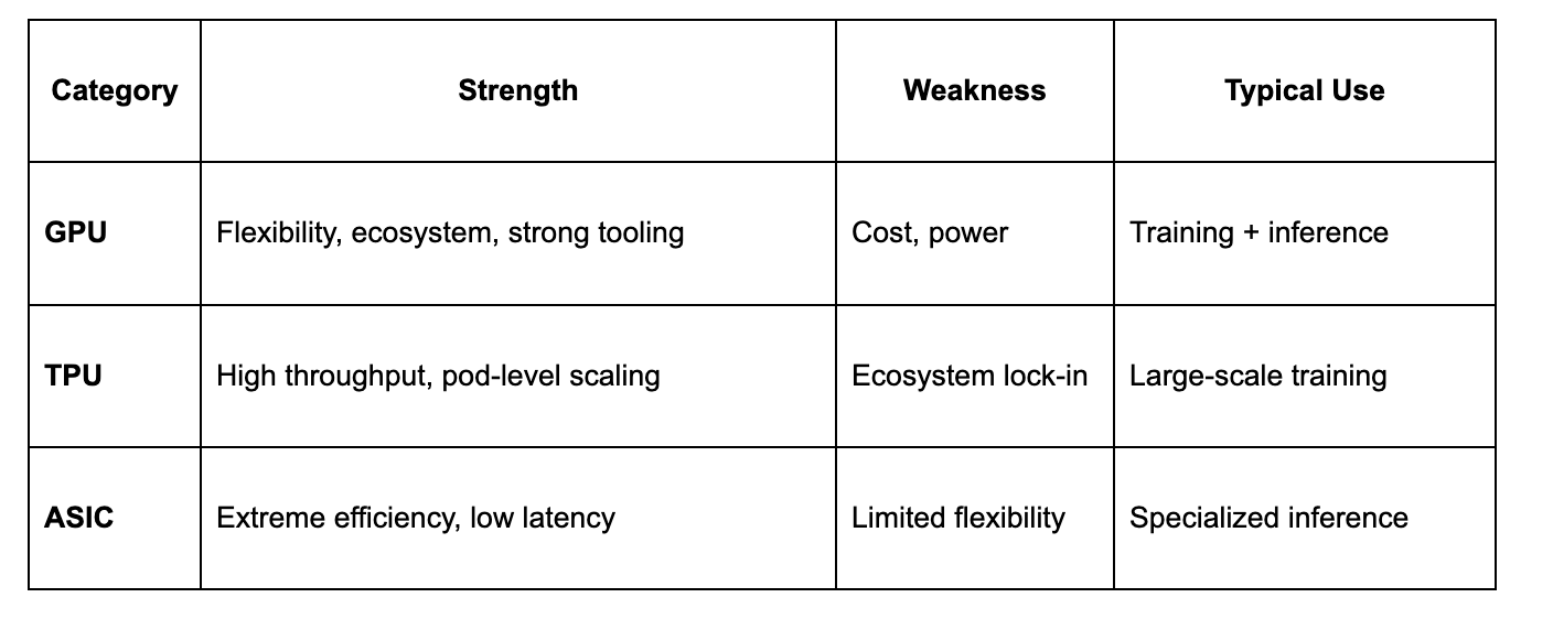
Modern AI systems run on specialized hardware designed to accelerate tensor computations. While the ecosystem is evolving rapidly, most AI workloads today run on three broad categories:

• GPUs (general-purpose accelerators)

• TPUs (cloud-scale tensor accelerators)

• AI ASICs (specialized accelerators)

High-Level Comparison

5.1 GPUs — The Default AI Compute Engine

Inside a Modern GPU

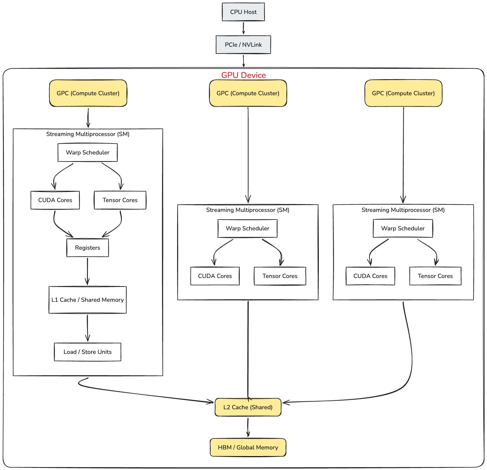
A modern GPU is organized as a hierarchy of parallel compute units designed to maximize throughput.

At the top level, the GPU consists of multiple compute clusters, each containing several Streaming Multiprocessors (SMs) — the core units where computation happens.

Each SM executes thousands of threads organized into warps (groups of 32 threads). These threads are scheduled by warp schedulers and executed on:

• CUDA cores for general computation

• Tensor cores for high-throughput matrix operations

Data flows through a multi-level memory hierarchy:

HBM → L2 Cache → L1 / Shared Memory → Registers → Compute

For AI workloads, performance depends on keeping compute units busy while minimizing data movement across memory levels.

Why GPUs Win:

• SIMT architecture → massive parallelism

• Mature ecosystem → CUDA, PyTorch, TensorRT

• Flexibility → supports diverse workloads

Used for:

• model training

• fine-tuning

• inference

Key Characteristics:

• High FLOPs (tensor cores)

• High-bandwidth memory (HBM)

• Strong software ecosystem

Limitation:

• Expensive

• Power-hungry

• Not always fully utilized

5.2 TPUs — Throughput at Scale

TPUs are Google’s custom accelerators designed for large-scale training.

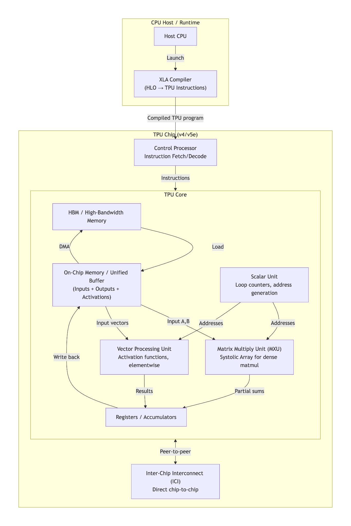
A TPU is designed around dense tensor computation. The key component is the Matrix Multiply Unit (MXU), often implemented using a systolic-array style dataflow.

Unlike GPUs, which are general-purpose parallel accelerators, TPUs are more tightly optimized for large matrix operations and compiler-driven execution through XLA.

Important path:

XLA graph → TPU Core → On-chip memory → MXU → HBM

Why TPUs Exist:

• Optimized for dense matrix multiplication

• Integrated with XLA compiler

• Designed for pod-level scaling

Strengths:

• High sustained throughput

• Efficient scaling across nodes

• Strong for large batch training

Limitations:

• Tight coupling with Google ecosystem

• Less flexible than GPUs

• Limited support for custom ops

5.3 AI ASICs — Extreme Specialization

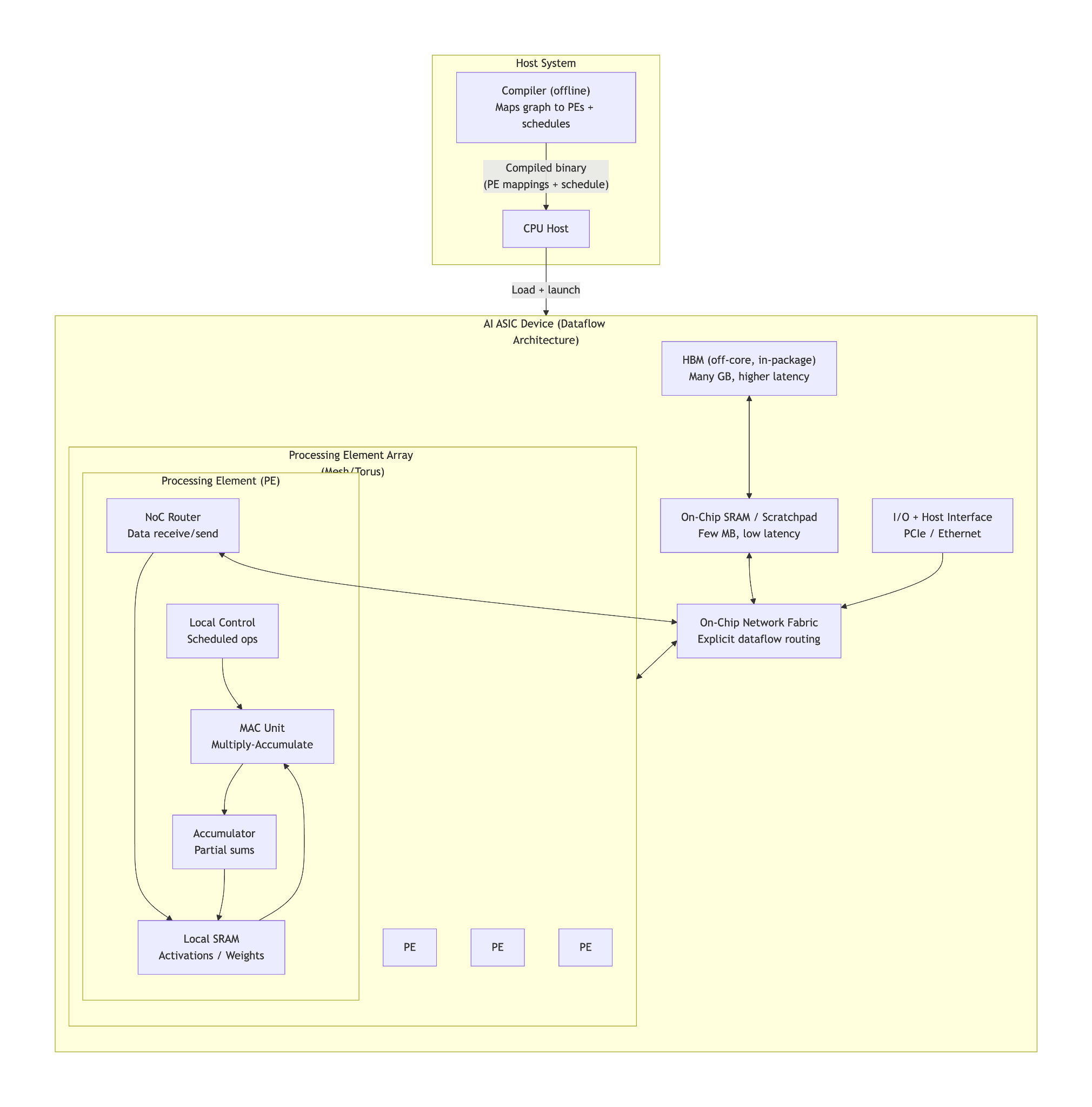
Above digram represent systems like Cerebras / Groq-style specialized accelerators

AI ASICs are designed for specialized efficiency. Instead of offering a broad programming model like GPUs, they usually optimize for a narrower execution pattern such as:

• dataflow execution

• low-latency inference

• large on-chip memory

• systolic / streaming compute

Important path:

Graph scheduler → dataflow fabric → processing elements → local memory

Examples:

• Cerebras (wafer-scale compute)

• Groq (low-latency inference)

Strengths:

• Very high efficiency

• Low latency (for inference)

• Optimized dataflow

Limitations:

• Limited programmability

• Narrow workload support

• Smaller ecosystem

5.4 Choosing the Right Hardware

The choice depends on workload:

Training

• GPU → general workloads

• TPU → large-scale dense training

Inference

• GPU → flexible, general-purpose

• ASIC → optimized, cost-efficient

At Scale

Hardware is used in combination:

• CPU → orchestration

• GPU → compute

• ASIC → specialized workloads

• Network → scaling

5.5 Key Trade-offs

Flexibility vs Efficiency

GPU → flexible but expensive

ASIC → efficient but limited

Ecosystem vs Optimization

GPU → strong ecosystem

TPU/ASIC → optimized pipelines

Choosing AI hardware is not just about picking GPUs vs TPUs vs ASICs.

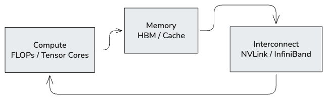
What actually determines performance are a small set of fundamental hardware characteristics:

• Compute (FLOPs)

• Memory (capacity + bandwidth)

• Interconnect (communication bandwidth + latency)

Understanding these is critical because:

AI systems fail when one of these becomes the bottleneck.

6.1 Compute — FLOPs Are Necessary, But Not Sufficient

Compute refers to the number of operations a system can perform per second.

• Measured in FLOPs (Floating Point Operations per second)

• Driven by:

  • CUDA cores

  • Tensor cores

Why Compute Matters

• Training large models requires massive matrix multiplications

• Higher FLOPs → faster training

But Compute Alone Is Not Enough

High FLOPs + poor memory = low utilization

Most real systems achieve only 30–60% of peak FLOPs

6.2 Memory — The Real Bottleneck in Modern AI

Memory is often the true limiting factor, especially for inference.

Two Key Aspects:

1. Capacity

• Model weights

• Activations

• KV cache

2. Bandwidth

• How fast data moves to compute units

• Critical for:

  • attention

  • inference

Why Memory Matters

If data cannot reach compute fast enough → compute stalls

Example

• Large LLM inference → memory-bound

• KV cache grows with sequence length

6.3 Interconnect — The Scaling Bottleneck

Interconnect determines how well systems scale across devices.

Types:

• NVLink (within node)

• InfiniBand / RoCE (across nodes)

Why It Matters

• Distributed training requires:

  • All-Reduce

  • All-Gather

Bottleneck

More GPUs ≠ faster training if communication is slow

6.5 Real-World Examples

Training Large Models

• Compute-heavy

• Communication-heavy

Bottleneck:

• interconnect + synchronization

LLM Inference

• Memory-heavy

• Latency-sensitive

Bottleneck:

• HBM bandwidth

• KV cache

6.6 How to Measure What Matters

Understanding compute, memory, and interconnect is useful — but in practice, performance tuning starts with measurement. Peak specs don’t matter. Utilization does.

Peak FLOPs ≠ Achieved FLOPs

Peak BW ≠ Achieved Bandwidth

6.6.1 Compute Utilization (MFU)

Model FLOPs Utilization (MFU)

MFU = (Actual FLOPs executed) / (Peak FLOPs)

• Measures how efficiently your model uses GPU compute

• Low MFU → compute underutilized

Rule of thumb:

< 30% → poor

30–60% → typical

> 60% → highly optimized

6.6.2 Memory Utilization

What to look for:

• Memory bandwidth usage

• Cache hit/miss patterns

• Memory stall time

Signal:

Low MFU + high memory usage → memory-bound system

Typical symptoms:

• GPU not fully utilized

• Increasing batch size has little effect

• Attention / KV cache workloads slow down

6.6.3 Interconnect / Communication

For distributed workloads:

Measure:

• All-Reduce / All-Gather time

• Compute vs communication ratio

• Network throughput

Signal:

Communication time ≥ compute time → interconnect bottleneck

6.6.4 Tools Engineers Actually Use

Quick Checks

nvidia-smi

• GPU utilization

• memory usage

• power

System Profiling

nsys profile python train.py

• end-to-end timeline

• CPU ↔ GPU interaction

Kernel-Level Profiling

nv-nsight-cu-cli

• kernel execution time

• memory throughput

• warp efficiency

Distributed Debugging

• NCCL debug logs

• PyTorch profiler (torch.profiler)

• TensorBoard traces

6.6.5 Bottleneck Diagnosis Cheat Sheet

• Low GPU util + low memory → pipeline / CPU bottleneck

• Low MFU + high memory → memory-bound

• High MFU + slow scaling → interconnect-bound

• High util + slow runtime → compute-bound

As AI systems scale, memory — not compute — often becomes the primary bottleneck, especially for large models and inference workloads.

Why Memory Matters

AI workloads constantly move data:

• Model weights

• Activations

• KV cache (in LLMs)

If data cannot reach compute units fast enough:

Compute stalls → performance drops

Two Critical Dimensions of Memory

1. Memory Capacity

• Determines how large a model you can run

• Includes:

  • model weights

  • activations

  • KV cache

2. Memory Bandwidth

• Determines how fast data moves

• Critical for:

  • attention

  • inference

  • real-time systems

As models scale beyond a single device, performance becomes a network problem.

Why Interconnect Matters

Large AI workloads are distributed across GPUs/nodes:

• Model parallelism

• Data parallelism

• Pipeline parallelism

This requires constant communication:

Compute → Communicate → Synchronize → Repeat

The Communication Bottleneck

Key operations:

• All-Reduce (gradients)

• All-Gather (activations / parameters)

At scale:

Communication time ≈ Compute time → poor scaling

Adding more GPUs does not guarantee speedup.

Types of Interconnects

Within Node

• NVLink

• NVSwitch

High bandwidth, low latency

Across Nodes

• InfiniBand

• RoCE

Lower bandwidth, higher latency

AI compute is evolving rapidly — not just in scale, but in how systems are designed and optimized.

The next phase of AI infrastructure will be shaped by a few key trends.

9.1 Memory Becomes the First-Class Constraint

As models grow larger and context lengths expand:

• KV cache dominates inference memory

• Activations dominate training memory

Memory footprint is growing faster than compute efficiency

Emerging directions:

• HBM4 and stacked memory architectures

• Memory compression (KV cache optimization)

• Model architectures designed for memory efficiency

9.2 Interconnect Becomes the New Bottleneck

Scaling beyond a single node exposes limits in communication:

• All-Reduce overhead

• Network contention

• Synchronization delays

Emerging directions:

• Faster interconnects (next-gen NVLink, InfiniBand)

• Optical interconnects

• Communication-aware model design

9.3 Efficient Compute: Precision & Sparsity

Raw FLOPs are no longer enough — efficiency matters.

Emerging directions:

• Lower precision formats (FP8, FP4, MX formats)

• Structured sparsity (e.g., 2:4 sparsity)

• Hardware–software co-design for efficient compute

9.4 Inference Becomes the Dominant Cost

At scale:

Inference cost > Training cost

Why:

• continuous usage

• real-time workloads

• large-scale deployments

Emerging directions:

• optimized inference runtimes (vLLM, TensorRT-LLM)

• batching and scheduling innovations

• model compression and distillation

9.5 Rise of System-Aware Model Design

Future models will not be designed in isolation.

Instead:

Model architecture ↔ hardware ↔ system constraints

Emerging directions:

• hardware-aware training

• communication-efficient architectures

• memory-efficient attention mechanisms

Modern AI systems can feel complex — spanning models, hardware, and distributed infrastructure.

But at their core, they can be understood through a simple mental model:

AI performance is constrained by three interacting factors:

Compute, Memory, and Interconnect

• Training → compute-heavy

• Inference → memory + latency-heavy

• Distributed systems → communication-heavy

What is limiting performance?

• Low GPU utilization → pipeline / memory issue

• High memory usage → memory-bound

• Poor scaling → interconnect-bound

So far, we’ve built a foundational understanding of AI compute:

• how hardware evolved

• how bottlenecks shifted from compute → memory → interconnect

• how modern AI systems are shaped by the entire stack

But we’ve only scratched the surface.

Knowing what limits performance is not enough —
the real challenge is understanding how to design systems that overcome those limits.

In Part 2, We Go Deeper

In the next part of this series, we will move from concepts to system design and optimization, including:

• Distributed training strategies
  (Data Parallel, Model Parallel, Pipeline Parallel)

• Inference systems at scale
  (batching, KV cache, scheduling)

• Communication optimization
  (All-Reduce, overlap, topology-aware scaling)

• Real-world system design trade-offs
  (latency vs throughput vs cost)