Princeton COS 597R “Deep Dive into Large Language Models” is a graduate course at Princeton University that systematically explores the principles of large language models, their preparation and training, architectural evolution, and applications in cutting-edge directions such as multimodality, alignment, tool use, and related issues. Note that this course focuses on conceptual understanding rather than engineering implementation.
I previously worked in distributed systems and database kernels, but in the past two years I moved to a large model company to work on data. These notes mainly consist of my organization and distillation of the course papers. What’s different is that I will combine some hands-on experience from solving practical problems at work, offering a bit of thinking from a career switcher’s perspective, hoping to help those who also want to enter algorithms from an engineering background.

This article comes from my paid column “System Thinking Daily”. Welcome to subscribe for more large model analysis articles; coupon information is at the end of the article.

This article mainly focuses on the foundational work of large models — Transformer.

First, we need to clarify the problem domain: what Transformer tries to solve is the sequence modeling problem, with the main representatives being language modeling and machine translation. Second, we need to know the problems existing in predecessor methods — RNN (Recurrent Neural Network) and CNN (Convolutional Neural Network) — in order to understand the innovation of Transformer. Finally, the key points of Transformer’s solution lie in the “multi-head attention mechanism” and “positional encoding”.

Author: Wood Bird Miscellany https://www.qtmuniao.com/2025/09/10/llm-1-transformer/ Please indicate the source when reprinting

Sequence Modeling

Sequence modeling is the modeling of an ordered sequence of elements to capture the dependency relationships (causality, the law of all things) between elements, so that we can:

1. Predict the next element in the sequence (language modeling)
2. Determine the validity of the sequence (grammar checking)
3. Transform one sequence into another (machine translation)

Sequence modeling is a rather generalized concept; many NLP tasks are essentially sequence modeling problems. Going further, many real-world automation problems can be transformed into sequence modeling problems.

Let’s look at some examples of sequence modeling to get a feel for it:

Domain	Form of Input/Output Sequence	Examples
Programming Language	Code token sequence	Code autocomplete, code translation, code generation
Molecular Structure	Chemical formula sequence (SMILES)	Drug generation
Image Captioning	Image → Description sequence	Summarizing image content
Multimodal Understanding	Image sequence + Text sequence	Q&A about image content, localization
Action Trajectory	GUI action sequence	Agent that automatically executes tasks

Therefore, with the success of large models, this method is now seen as one of the most promising paths toward AGI.

Predecessor Solutions

Below we look at the main problems of traditional recurrent structures (RNN/LSTM) and convolutional structures (CNN) when performing sequence modeling.

Recurrent Structures

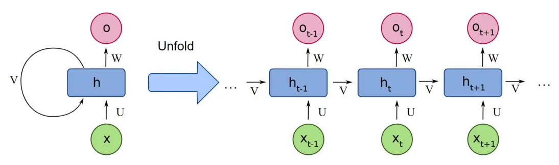
Recurrent structures such as RNN / LSTM / GRU once dominated sequence modeling for a long time. Their formula is:

$$
h_{t}=f(h_{t-1},x_{t})
$$

We can use images to aid understanding:

transformer-rnn.png

Where $h_{t}$ is the hidden state at position t (or “time step”), and $x_{t}$ is the input at position t. Intuitively, it’s easy to understand: it compresses the previous input sequence into a hidden state $h_{t}$ and passes it backward step by step. From the circles in the figure, we can better understand why it’s called a recurrent structure.

This structure mainly has two problems:

1. Cannot perform parallel computation
2. Long-distance information dilution

It can be seen that in this structure, the computation of each hidden state ($h_{t}$) depends on the previous result ($h_{t-1}$). This sequential dependency means that when we want to get the final state, we can only compute step by step in series. Therefore, we cannot fully utilize the parallel capability of GPUs, and training becomes very slow as soon as the network grows slightly larger.

In addition, the state transfer between different elements all depends on such step-by-step computation. It is conceivable that when the distance is far enough, the information of elements at the front of the sequence will be diluted to what extent. Therefore, RNN structures find it difficult to capture dependencies between two words that are too far apart.

Convolutional Structures

Convolutional Neural Networks (CNN) shone brilliantly in the previous wave of AI where computer vision was the main application field. The core characteristics are its parallelism and deep stackability (of course, mainly relying on techniques such as residual networks created in the same period), thereby building sufficiently complex network structures to accommodate enough information.

Therefore, CNNs were introduced into sequence modeling, represented by ByteNet, ConvS2S, attempting to parallelize modeling through local receptive fields + multi-layer stacking. But CNNs also have their problems:

1. Single-layer convolution has limited receptive field
2. Cannot capture absolute position information

Since a single convolutional kernel is usually not too large (for example, in images, convolutional kernels are usually 3×3 or 5×5; too large doesn’t work well), to capture long-distance dependencies, multiple layers are usually stacked to expand the receptive field. But networks that are too deep not only make training harder, but also greatly increase training costs. The essence is that convolution is relatively inefficient for long-distance modeling.

Unlike images, for sequences, we usually perform one-dimensional convolution along the position or time dimension. Since the convolutional kernel is essentially position-agnostic (no position information, just weights; left and right parameters are the same), it can only capture relative position information within the kernel’s field of view. In addition, a major reason why convolution works well in the image domain is: translation invariance. For example, a cat appearing in the upper-left corner and lower-right corner is still a cat. But in language sequences, the meaning of a word is highly context-dependent. Therefore, convolution is not a native structure for sequences.

Core Architecture

After analyzing the problem domain and the shortcomings of predecessor solutions, let’s see how Transformer designs the network structure to solve these two problems. But before going into detail, let’s lay some groundwork with related concepts.

Encoder-decoder structure. This was proposed to solve the seq2seq class of problems in sequence modeling that we mentioned earlier, mainly applied in neural network-based machine translation. When first proposed (2014), it was based on RNN.

Its basic working principle is:

1. The encoder encodes the input sequence into a fixed-length context vector. Intuitively, this vector is similar to a “summary” of the input sentence.
2. The decoder uses this context vector as the initial hidden state and generates the output sequence step by step in an “auto-regressive” manner.

Therefore, the initial encoder-decoder structure bridges the input and output sequences through a fixed-length intermediate vector. It is conceivable that when the information volume of the input sequence increases (for example, the sequence becomes longer), this fixed-length “bridge” will become a bottleneck.

Auto-regressive. Auto-regression was originally a concept in statistics and time series analysis. Its basic meaning is that the current value of a variable equals a linear combination of past values, plus a random disturbance term. In large models, when outputting the next token, the model feeds the already output tokens as context into the model together.

For example, when GPT generates the sentence “The sky is blue”:

• First generate “The sky”.
• Then use “The sky” as context to generate “is”.
• Then use “The sky is” as context to generate “blue”.
• Finally use “The sky is blue” as context to generate “的” (or the final token).

There will be some redundant information in this process, which is also a key direction that inference infra focuses on: KV Cache. Of course, the KV concept here involves some concepts of Attention, which will be expanded upon later.

Self-attention. The attention mechanism was initially introduced to solve the “information bottleneck” problem of the intermediate bridging vector in the encoder-decoder structure. Its basic approach is:

1. During encoding: (finer granularity) Instead of encoding the entire input sequence into a fixed-length vector, generate a “relationship” vector for each word. This vector contains the “closeness” relationship between this word and other words in the sequence. Of course, the position information of this word is also encoded in some way.
2. During decoding: (distinguishing closeness) When generating each word, it no longer relies solely on a fixed-length context vector, but dynamically attends to different parts of the input sequence. In implementation, it uses the previously obtained “relationship” vector of each word to weight the input sequence according to “attention” (closeness) to get the next word.

To put it figuratively, the attention mechanism:

1. Finer granularity: Instead of generating a “summary” for the entire input sequence, generate a summary for each word individually.
2. Distinguishing closeness: Instead of crudely using a fixed-length context for decoding, dynamically obtain the parts of the input sequence that should be most focused on at each decoding step, and perform weighting.

Architecture

transformer-architecture.png

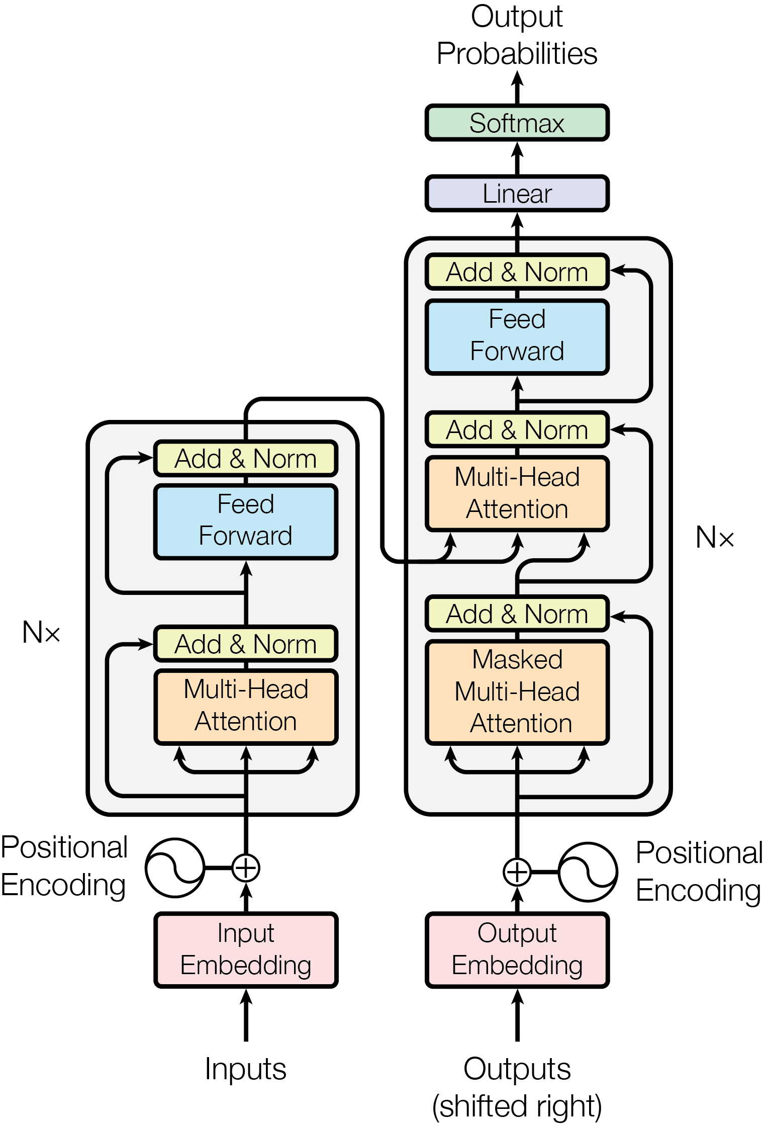
With the above groundwork, let’s look at this classic Transformer architecture diagram from the paper.

The main trunk’s left and right sides follow the classic encoder-decoder structure.

On the encoder side, N=6 basic layers are stacked. During stacking, residual connections and normalization (Add & Norm) are used to avoid the vanishing and exploding gradient problems of deep neural networks. Each basic layer contains two basic units: Multi-Head Attention and Feed Forward. The feed-forward network is actually a three-layer fully connected network with one hidden layer. We will analyze these two basic building blocks in detail later.

The decoder structure on the right is largely the same as the encoder’s basic structure, with the same number of layers, but with two changes. First, a cross-attention module is added to bridge the “context” extracted by the encoder. Second, the attention computation must first be masked, so that each word can only attend to words before it, and cannot see words after it.

Finally, it goes through a linear layer, and then softmax is used for probability normalization.

In addition, the input can also be divided into two parts:

1. Token to vector conversion: the tokenizer is not shown here. The token-to-vector conversion function can also be learned.
2. Superimposing position information: superimpose the position information of each token in the sentence onto its vector.

Attention

When computing attention, we introduce three additional representations for each token’s vector: Q (query), K (key), V (value). That is, from the original token vector (let’s call it x), three representations with different purposes are extracted (or derived) through “projection” (matrix transformation) in another space. Below, we use an example of “looking up materials in a library” to understand this.

Imagine you need to write a paper on “The Impact of Artificial Intelligence on the Economy” and need to look up some relevant literature in the library.

• Original input vector (x): Like a vague idea in your mind or a highly abstract word, such as “economy”. This idea itself contains many dimensions of meaning.
• Query (Q): To find materials, you can’t just hold onto the vague idea of “economy”. You need to make it concrete into a question or query, such as “Find books about how AI technology changes the employment market”. This specific query is Q. It is derived from your original idea “economy”, but more directional.
• Key (K): In the library, so that every book can be quickly retrieved, each book has its own labels or keywords, such as “AI”, “employment”, “automation”, “market analysis”, etc. These labels are K. They represent the summary of the book and are used for relevance matching with the “query”.
• Value (V): The actual content of the book is V. Once your query (Q) highly matches a book’s label (K), you can read the detailed content (V) of that book to get more information.

Then why not just directly use the original vector x to multiply with other tokens’ vectors? There are several reasons:

1. Role decoupling: If QKV all use x, then this vector needs to “play three roles” at the same time, which is actually a strong prior constraint. This is more obvious in cross-attention.
2. Expressiveness: Projecting the original vector into different spaces is essentially a more cohesive extraction, and this extraction method can also be parameterized and learned, thus greatly improving flexibility and expressiveness.
3. Supporting multi-head: Precisely because the same x can have different “extraction” methods, Transformer’s multi-head parallel extraction of features from different dimensions makes sense.

Transformer uses two types of attention:

1. Self-attention: The attention layer in the encoder part, capturing the intrinsic dependency relationships among tokens in the sequence. At this time, QKV all come from different projections of the same sequence.
2. Cross-attention: The bridging part between encoder and decoder, utilizing the intrinsic dependency relationships captured by the encoder to predict the next token. At this time, Q comes from the decoder, and KV comes from the encoder.

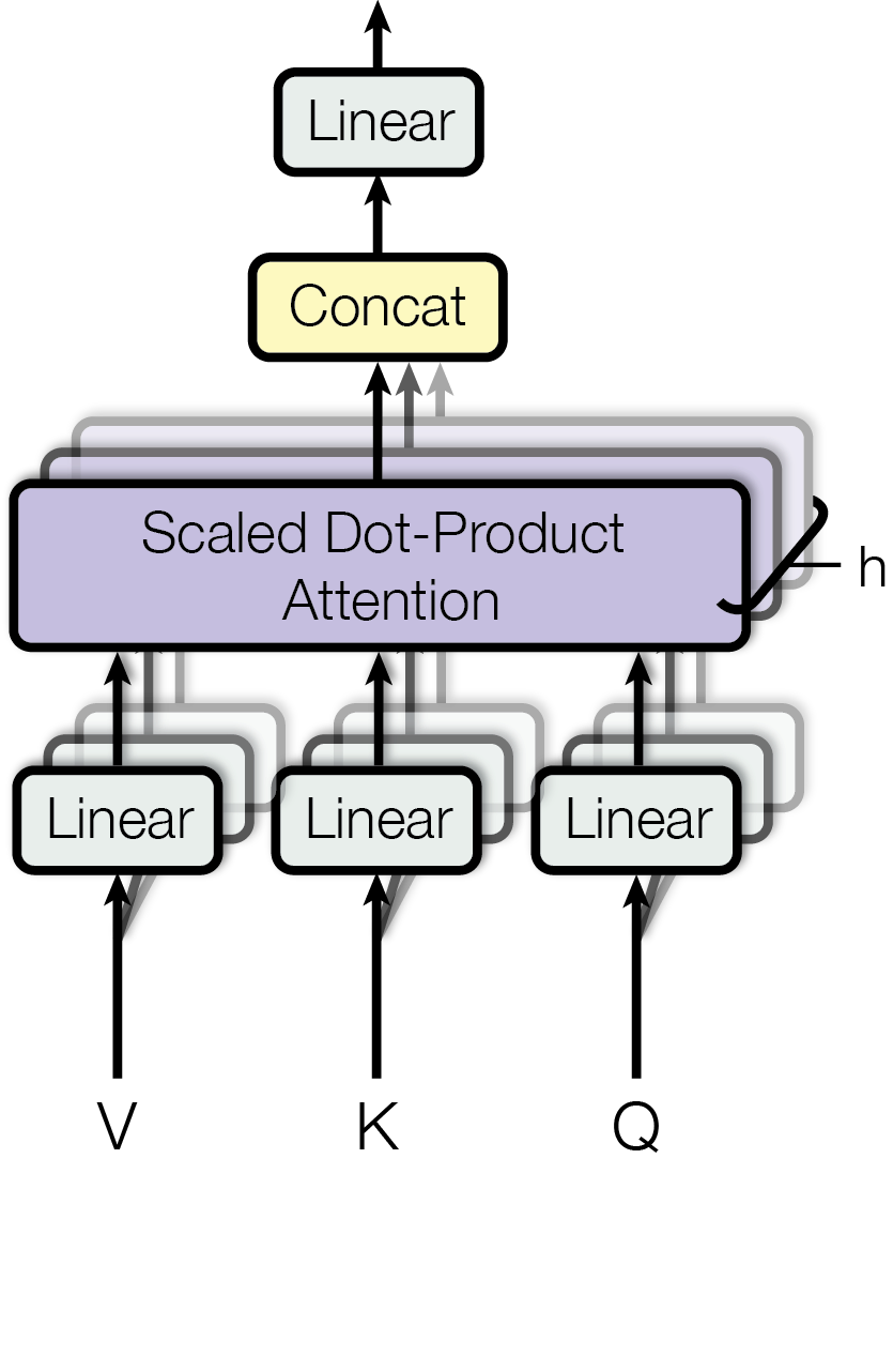
Within the given window, the attention module computes the correlation between each token and other tokens, thereby obtaining a relationship vector for each token with respect to all other tokens. When computing correlation, additive attention or dot-product (multiplicative) attention can be used. The effects are similar, but because GPUs are highly optimized for dot products, the latter is chosen. Finally, to maintain output distribution stability (after dot product, the mean will be amplified by $\sqrt{d_k}$ — you can check the dot product formula to see this), a scaling (dividing by $\sqrt{d_k}$) is added to bring the mean back, to avoid pushing the softmax function into a region with extremely small gradients.

transformer-vqa.png

Then why use multiple heads? This actually borrows from the characteristics of Convolutional Neural Networks (CNN) — multi-head extraction and deep stacking — to extract features from different dimensions respectively, and finally recombine them using a linear layer, achieving better results.

The paper uses h=8 parallel attention layers, or heads. For each head, $d_{k} = d_{v} = d_{model} / h = 64$, that is, while increasing the number of heads, the dimension of each head is reduced. Thus, while keeping the computational volume roughly the same, multiple features can be extracted in parallel.

Feed-Forward Network Layer (FFN)

This is a three-layer fully connected neural network (input layer, hidden layer, output layer). Similar to the combination layer with convolution kernel = 1 after multiple heads in CNN, it provides additional non-linearity (mainly through the activation function). Intuitively, the self-attention layer integrates information “horizontally” (across tokens within the window), aggregating contextual information from all relevant words into each token’s representation. The FFN layer deepens and refines this aggregated information “vertically” (without interaction between words, along the feature dimensions within each word). It independently performs feature learning and reshaping at each position, enabling it to better capture more abstract, higher-level features at that position.

Positional Encoding

Since the attention module computes the relative relationships between different tokens in the sequence, it has no position information. To allow the network to learn positional information between tokens, that is, the causality we mentioned earlier, Transformer additionally introduces positional encoding. To allow positional encoding to be easily superimposed onto the token’s embedding, it maintains the same dimension as the embedding, 512. Thus, simple addition can be used for superposition.

This encoding can be learned through parameters, or fixed in advance. Transformer chose the latter, because it was found to be about the same as learned ones (but of course, subsequent works have made extensive improvements). Transformer adopted a sinusoidal encoding method, whose characteristic is that it can capture the additivity of positions.

Summary

This article first clarifies the problem domain — sequence modeling, discusses why sequence modeling can become the foundation for solving a large class of general problems; then briefly analyzes some problems existing in previous RNN and CNN: difficulty in parallelization and long-distance dependency capture; finally analyzes Transformer’s solution and main architecture — the multi-head self-attention mechanism.

In addition, we can trace the transformation process of an embedding corresponding to a token (the dimension remains 512 throughout the transformation) to gain a deeper understanding of Transformer.

Encoder part:

1. Positional encoding: addition, superimposing position information
2. Self-attention layer: capturing relationships among token vectors in the input sequence and compressing them into representation vectors (looking both ways)
3. FNN linear layer: adding some non-linearity, tempering each token’s representation vector

Decoder part:

1. Masked self-attention layer: capturing dependencies between each token in the output sequence and its preceding tokens, compressing them into representation vectors (only looking forward)
2. Cross-attention: sending the learned correlation representations of tokens in the input sequence to the decoder, so that the new representation vector contains both information from the input sequence and information from preceding tokens in the output. Thus preparing all the information needed to predict the next token.
3. FNN linear layer: tempering each token’s representation vector, adding some non-linearity

Multi-layer stacking: through residuals and normalization, to deepen the network while maintaining training stability. Thus performing repeated extraction and refinement, using more parameters to accommodate more information.

---