ray.data is a wrapper layer built on top of ray core. With ray.data, users can implement large-scale heterogeneous data processing (mainly using both CPU and GPU) with simple code. In one sentence: it’s simple and easy to use, but also has many pitfalls.
In the previous post, we started from the user interface and briefly outlined the main APIs of ray.data. In this post, we will take a macroscopic view and roughly go through the basic principles of ray.data. After that, we will use a few more posts, combined with code details and practical experience, to discuss several important topics: execution scheduling, data formats, and a pitfall avoidance guide.
This article comes from my column “System Thinking Daily”. If you find the article helpful, welcome to subscribe to support me.

Overview

From a high-level understanding, a ray.data processing task can be roughly divided into three sequential stages:

1. Data Loading: Reading data from external systems into Ray’s Object Store (e.g., read_parquet)
2. Data Transformation: Using various operators to transform data in the Object Store (e.g., map/filter/repartition)
3. Data Write-back: Writing data from the Object Store back to external storage (e.g., write_parquet)

Author: Muniao’s Notes https://www.qtmuniao.com/2024/07/07/ray-data-2/ Please indicate the source when reposting

ray-object-store.png

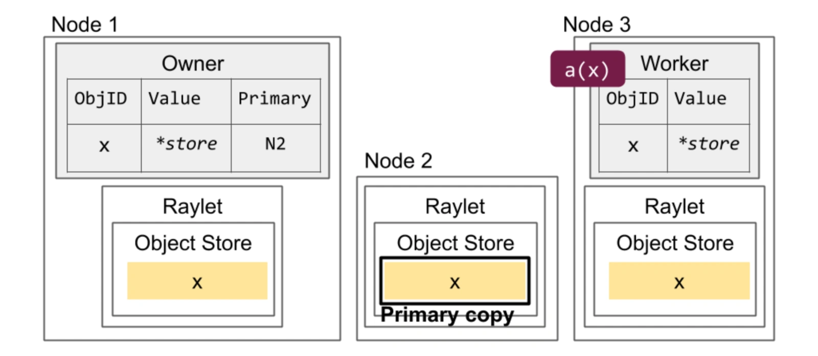
As shown in the figure above, let me explain the mentioned terms:

• Object Store is composed of controlled memory on each node, used to store intermediate results from the previous subtask for the next subtask on other nodes to pull and use.
• Raylet is the daemon of ray on each node in the cluster, responsible for scheduling and executing various ray tasks on that node.

Data Abstraction

ray.data uses three levels of granularity to organize a dataset: Dataset, Block, and Row. Each dataset is logically a two-dimensional table; after being read into the system, it is split into multiple blocks distributed across multiple machines’ Object Stores.

Among them, blocks are immutable and are the basic unit for ray.data to store and transmit data, as well as the most basic parallel granularity. Blocks are stored in the Object Store in Apache Arrow format, which features columnar storage, language independence, and zero-copy support.

batch, not block

There is a very important vectorized (batch is organized by columns and passed to operators) processing operator in ray data: map_batches. We can get a rough sense of its usage through an example:

1
2
3
4
5
6
7
8
9
10
11
12
13
14
15
16
17

from typing import Dict
import numpy as np
import ray

def add_dog_years(batch: Dict[str, np.ndarray]) -> Dict[str, np.ndarray]:
    batch["age_in_dog_years"] = 7 * batch["age"]
    return batch

ds = (
    ray.data.from_items([
        {"name": "Luna", "age": 4},
        {"name": "Rory", "age": 14},
        {"name": "Scout", "age": 9},
    ])
    .map_batches(add_dog_years, batch_size=32)
)
ds.show()

This operator involves a batch parameter. This batch and block are decoupled; their differences and connections are:

1. block is a physical static storage entity; while batch is dynamically generated before data is sent to the operator.
2. ray.data will combine one or more blocks into a batch_size and send it to the user’s operator.
3. After processing, each batch becomes a new block and is written back to the Object Store.

Note the last step: the output of a batch after processing is not necessarily one block, because ray data has control over block size: [1M, 128M] (can be modified via DataContext.target_min_block_size and DataContext.target_max_block_size); if too large, it will be split, but if too small, it seems not to be merged.

Initial Number of Blocks

After discussing the relationship between block and batch, we can easily think of a question: after a dataset is loaded into memory, how many blocks will it be divided into?

First, we can explicitly specify the number in read-like operators: override_num_blocks

1
2
3
4
5
6

import ray

ray.init(num_cpus=2)

ds = ray.data.read_csv("example://iris.csv", **override_num_blocks**=1).map(lambda row: row)
print(ds.materialize().stats())

Second, if we do not specify, ray data will estimate based on a series of rules. The rough estimation steps are:

1. Initial Size: The initial block count is 200
2. Size Constraint Adjustment: Sampling roughly estimates the total size to select an appropriate number of blocks, ensuring a single block size falls within the [1M, 128M] range
3. Parallelism Constraint Adjustment: Considering the number of available CPUs, to fully utilize CPUs during data loading — ensuring the block count is at least twice the number of CPU cores

The last item involves an implementation detail: ray.data will schedule one read task for each block, that is, as we mentioned before, block is the basic parallel unit.

Number of Blocks Written to Files

If no control is applied, when persisting a dataset to external systems, each block will by default be written as one file. If you want to change the number of files, for example, to avoid too many small files, you can use the Repartition operator to change the number of blocks:

1

Dataset.repartition(num_blocks: int, *, shuffle: bool = False) → Dataset[source]

Weak Schema

We mentioned earlier that logically a dataset (Dataset) can be understood as a large two-dimensional table, but unlike relational databases where each column type is strongly constrained, ray data only applies weak constraints to the columns in the dataset. After all, this is Python…

This design indeed gives users a lot of flexibility, but also brings a lot of pitfalls, just like the Python language itself — how well it works depends entirely on the user’s skill level.

But paradoxically, ray.data datasets do have a schema interface; it’s just inferred by reading the first row. As in the code below, for the age column, when both string and integer types exist simultaneously, ray.data will not report an error, and instead takes the data type of the first row as the type for that column.

1
2
3
4
5
6
7
8
9
10
11
12
13
14
15
16
17
18
19
20
21
22
23
24
25
26
27
28
29
30

def add_dog_years(batch: Dict[str, np.ndarray]) -> Dict[str, np.ndarray]:
    batch["age_in_dog_years"] = 7 * batch["age"]
    return batch

ds = (
    ray.data.from_items([
        {"name": "Luna", "age": "3"},
        {"name": "Rory", "age": 14},
        {"name": "Scout", "age": 12},
    ])
    .map_batches(add_dog_years)
)

print(ds.schema())









ds.show()

batch organizes data by columns, that is, the type of batch is Dict[str, np.ndarray], with each column organized using numpy. But if each value in the np.ndarray is None, nested, or of variable length, ray will not perform any checks; the user has to guarantee it themselves.

This leads to a lot of pitfalls in practice, including:

1. numpy does not support Python’s None type. Therefore, if new data after processing is mixed with None, before converting to a block and storing it in the object store, it will take a detour — first converting to Pandas, then to Arrow, and then writing to the Object Store.
2. If the output of a column in a batch is a high-dimensional numpy array, ray will wrap it into a custom ArrowTensorArray, pretending it is a multi-row numpy array, but the memory is still organized as a high-dimensional numpy array.

These various implicit conversions bring a lot of trouble to new users.

Essentially, ray.data does not have its own type system; instead, it uses numpy, pandas, and pyarrow to construct a type system and its serialization/deserialization methods. But when used together, there are many frictions, leading to a lot of bugs with unexpected behavior. For this reason, ray.data is constantly iterating and frantically patching, often releasing a minor version every few weeks.

Task Execution

So how does ray.data perform large-scale parallel execution of a pipeline? It can be briefly summarized in two words:

1. micro-batch mode
2. operator parallelism (operator-pool)

Task Types

To elaborate, ray.data builds a pipeline composed of operators based on the user’s definition. For each operator in the pipeline, it launches a corresponding number of Tasks or Actors based on the user-configured parallelism:

1. Task: For stateless functions passed by the user, destroyed immediately after the call. For example, a very simple map that increments a count
2. Actor: For stateful classes passed by the user, resident in memory. For example, inference in a map that requires pre-loading a model. Using Actor mode, the model only needs to be loaded once in the constructor, and then multiple batches can be inferred until the entire task is completed.

Scheduling Logic

After launching the execution units (Task or Actor) for all operators, the basic scheduling logic of ray.data is:

1. Maintain an input buffer and an output buffer for each operator, storing references to blocks (the blocks themselves are in the object store)
2. For all operators, when there is data in the input buffer, a task (task or actor) is scheduled to consume it and place it in the output buffer
3. The input offer of the downstream operator is the output buffer of the upstream operator

That is, all operators are logically bridged through blocking queues (input/output buffers), and according to the parallel granularity specified by the user for each operator, tasks are scheduled to drive the data to flow forward as a whole.

And when the data is almost processed, Actors that are no longer needed by earlier operators in the pipeline will be released (Tasks are stateless and released immediately after the call, while Actors are resident).

In newer versions, Task and Actor also support configuring dynamic parallelism ranges, and ray data can perform elastic scheduling based on resources and demands, but the implementation is still very rough and the actual experience is not ideal.

In addition, ray.data will also perform a certain amount of backpressure on the execution of upstream operators based on the memory usage of the downstream Object Store. But if your downstream operator’s memory usage is not in the Object Store but in the process’s heap, then ray is powerless.

Limitations

ray.data is not suitable for large-scale shuffle. Here is a rough definition of shuffle: multi-to-multi data exchange between multiple nodes. For example, operators like sort and rand_shuffle.

Unlike Spark, ray.data needs to load all data into memory before performing a shuffle. Therefore, if the data volume is large and cannot fit in memory, a large amount of spill will occur. But ray.data manages spilled data on external storage very poorly, and various optimizations in shuffle (such as pre-sorting, small file merging) are also done very poorly. Therefore, for most shuffle scenarios, Ray is not as fast as Spark.

Not to mention, Ray does not support the Join operator at the interface level (which is also a very common shuffle operator).

Summary

This article has described at a macro level ray.data’s organization and transformation of blocks, its handling of data schemas, and its basic execution scheduling logic. In the future, we will delve into the code details and talk about ray.data’s execution engine.