Natural Language Processing has undergone a massive evolution in recent years. To understand state-of-the-art models, we first need to look back at how we used to process sequences and the critical bottleneck that led to the invention of Attention.

The Foundation: Seq2Seq with RNNs

In traditional Sequence-to-Sequence (Seq2Seq) models—commonly used for tasks like machine translation—the architecture relies on Recurrent Neural Networks (RNNs) and consists of two main components:

• Encoder RNN: Processes the input sequence x=(x1,x2,…,xT)x = (x_1, x_2, \dots, x_T) and produces a sequence of hidden states h=(h1,h2,…,hT)h = (h_1, h_2, \dots, h_T).
• Decoder RNN: Generates the output sequence y=(y1,y2,…,yT′)y = (y_1, y_2, \dots, y_{T'}) step by step.

The encoder’s final hidden state hTh_T is passed as the initial hidden state of the decoder. This vector—often called the context vector—carries a heavy burden: it must encode all necessary information from the entire input sequence.

The Context Bottleneck
When dealing with long input sequences, a single fixed-size context vector struggles to capture all relevant details. Information inevitably gets lost or diluted, leading to poor model performance on longer text.

The Solution: The Attention Mechanism

To overcome the context bottleneck, the attention mechanism was introduced. It allows the decoder to dynamically focus on different parts of the input sequence at each decoding step, rather than relying on a single static vector.

How It Works Step-by-Step

At decoder timestep tt, the model performs the following operations:

1. Compute Alignment Scores: Calculate the relevance between the current decoder state st−1s_{t-1} and each encoder hidden state hih_i:

eti=fattn(st−1,hi)e_{ti} = f_{\text{attn}}(s_{t-1}, h_i)

A common mathematical choice for this is:

eti=va⊤tanh⁡(Wa[st−1;hi])e_{ti} = v_a^\top \tanh(W_a [s_{t-1}; h_i])

(Where WaW_a and vav_a are learnable parameters, and [⋅;⋅][\cdot;\cdot] denotes concatenation).
2. Normalize Scores: Use a softmax function to convert the scores into probabilities (attention weights):

αti=exp⁡(eti)∑j=1Texp⁡(etj)\alpha_{ti} = \frac{\exp(e_{ti})}{\sum_{j=1}^T \exp(e_{tj})}

3. Compute the Context Vector: Create a weighted sum of the encoder hidden states using the attention weights:

ct=∑i=1Tαtihic_t = \sum_{i=1}^T \alpha_{ti} h_i

4. Decode: Use the new, time-dependent context vector ctc_t in the decoder. This is typically done by concatenating ctc_t with the decoder input yt−1y_{t-1}, or feeding [ct;st−1][c_t; s_{t-1}] directly into the output layer to predict yty_t.

Key Advantages of Attention

• Dynamic Focus: The model attends to the most relevant input tokens for each specific output step.
• No Fixed Bottleneck: The full input sequence remains accessible throughout the entire decoding process.
• Fully Differentiable: Attention weights are learned end-to-end via backpropagation, requiring no external supervision for alignment.

Generalizing to Attention Layers

In the Seq2Seq model, we can think of the decoder RNN states as Query Vectors and the encoder RNN states as Data Vectors. These get transformed to output Context Vectors. This specific operation is so powerful that it was extracted into a standalone, general-purpose neural network component: the Attention Layer.

To prevent vanishing gradients caused by large similarities saturating the softmax function, modern layers use Scaled Dot-Product Attention. Furthermore, separating the data into distinct “Keys” and “Values” increases flexibility, and processing multiple queries simultaneously maximizes parallelizability.

The Inputs

• Query vector QQ [Dimensions: NQ×DQN_Q \times D_Q]
• Data vectors XX [Dimensions: NX×DXN_X \times D_X]
• Key matrix WKW_K [Dimensions: DX×DQD_X \times D_Q]
• Value matrix WVW_V [Dimensions: DX×DVD_X \times D_V]

(Note: The key weights, value weights, and attention weights are all learnable through backpropagation).

The Computation Process

1. Keys: The data vectors are projected into the key space.

K=XWK[NX×DQ]K = X W_K \quad [N_X \times D_Q]

2. Values: The data vectors are projected into the value space.

V=XWV[NX×DV]V = X W_V \quad [N_X \times D_V]

3. Similarities: Calculate the dot product between queries and keys, scaled by the square root of the query dimension.

E=QKT/DQ[NQ×NX]E = Q K^T / \sqrt{D_Q} \quad [N_Q \times N_X]

Eij=Qi⋅Kj/DQE_{ij} = Q_i \cdot K_j / \sqrt{D_Q}

4. Attention Weights: Normalize the similarities using softmax along dimension 1.

A=softmax(E,dim=1)[NQ×NX]A = \text{softmax}(E, \text{dim}=1) \quad [N_Q \times N_X]

5. Output Vector: Generate the final output as a weighted sum of the values.

Y=AV[NQ×DV]Y = A V \quad [N_Q \times D_V]

Yi=∑jAijVjY_i = \sum_j A_{ij} V_j

Flavors of Attention

Depending on how we route the data, attention layers take on different properties:

• Cross-Attention Layer: The data vectors and the query vectors come from two completely different sets of data.
• Self-Attention Layer: The exact same set of vectors is used for both the data and the query. Because self-attention is permutation equivariant (it doesn’t inherently know the sequence order), we must add positional encoding to inject position information into each input vector.
• Masked Self-Attention: We override certain similarities with negative infinity (−∞-\infty) before the softmax step. This strictly controls which inputs each vector is allowed to “look at” (often used to prevent looking into the future during text generation).
• Multi-Headed Attention: We run HH copies of Self-Attention in parallel, each with its own independent weights (called “heads”). We then stack the HH independent outputs and use a final output projection matrix to fuse the data together.

The Rise of Transformers

Under the hood, self-attention boils down to four highly optimized matrix multiplications. However, calculating attention across every token pair requires O(N2)O(N^2) compute.

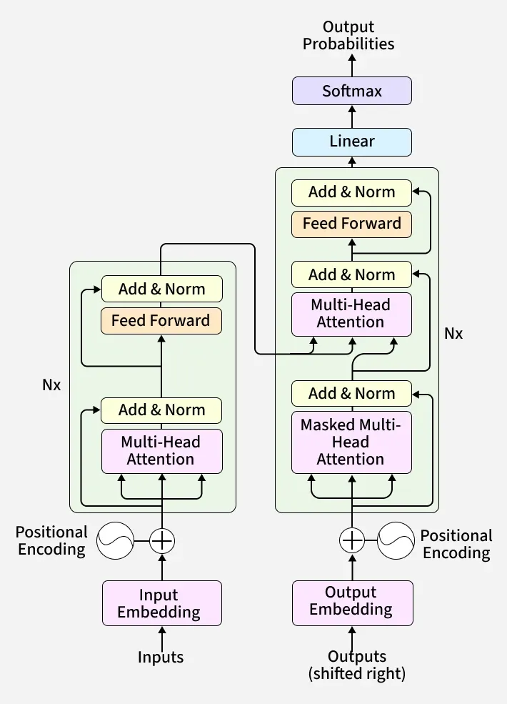
By taking these attention layers and building around them, we get the modern Transformer:

The Transformer Block
A single block consists of a self-attention layer, a residual connection, Layer Normalization, several Multi-Layer Perceptrons (MLPs) applied independently to each output vector, followed by another residual connection and a final Layer Normalization.

Because they discard the sequential nature of RNNs, Transformers are incredibly parallelizable. Ultimately, a full Transformer Model is simply a stack of these identical, highly efficient blocks working together to process complex sequential data.

Applications

The true power of the Transformer lies in its versatility. By simply changing how data is pre-processed and fed into the model, the exact same attention mechanism can solve vastly different problems.

Large Language Models (LLMs)

Modern text-generation giants (like GPT-4 or Gemini) are primarily built on decoder-only Transformers. Here is how the pipeline flows:

1. Embedding: The model begins with an embedding matrix that converts discrete words (or sub-word tokens) into continuous, dense vectors.
2. Masked Self-Attention: These vectors are passed through stacked Transformer blocks. Crucially, these blocks use Masked Multi-Headed Self-Attention. The mask prevents the model from “cheating” by looking at future words, forcing it to learn sequence dependencies based only on past context.
3. Projection: After the final Transformer block, a learned projection matrix transforms each vector into a set of scores (logits) mapping to every word in the model’s vocabulary. A softmax function converts these into probabilities to predict the next word.

Vision Transformers (ViTs)

Who says Transformers are only for text? In 2020, researchers proved that the exact same architecture could achieve state-of-the-art results on images.

1. Patching: Instead of tokens, a ViT breaks an image down into a grid of fixed-size patches (e.g., 16x16 pixels).
2. Flattening: These 2D patches are flattened into 1D vectors and passed through a linear projection layer.
3. Positional Encoding: Because the model processes all patches simultaneously, positional encodings are added to retain the image’s 2D spatial relationships.
4. Unmasked Attention: Unlike LLMs, ViTs use an encoder-only architecture. There is no masking—the model is allowed to attend to the entire image at once to understand global context.
5. Pooling: At the end of the transformer blocks, the output vectors are pooled (or a special [CLS] classification token is used) to make a final prediction about the image.

Modern Architectural Upgrades

The original “vanilla” Transformer from the 2017 Attention is All You Need paper is rarely used exactly as written today. Researchers have introduced several key modifications to make models train faster, scale larger, and perform better.

Pre-Norm (vs. Post-Norm)

The original Transformer applied Layer Normalization after adding the residual connection (Post-Norm). Modern architectures apply it before the Attention and MLP blocks (Pre-Norm). This seemingly minor change drastically improves training stability, allowing researchers to train much deeper networks without the gradients blowing up or vanishing.

RMSNorm (Root Mean-Square Normalization)

Standard Layer Normalization is computationally expensive because it requires calculating the mean to center the data. RMSNorm is a leaner alternative that drops the mean-centering step entirely, scaling the activations purely by their Root Mean Square. This makes training slightly more stable and noticeably faster.

Given an input vector xx of shape DD, and a learned weight parameter γ\gamma of shape DD, the output yy is calculated as:

yi=xiRMS(x)∗γiy_i = \frac{x_i}{RMS(x)} * \gamma_i

Where the Root Mean Square is defined as:

RMS(x)=ϵ+1N∑i=1Nxi2RMS(x) = \sqrt{\epsilon + \frac{1}{N} \sum_{i=1}^N x_i^2}

(Note: ϵ\epsilon is a very small number added to prevent division by zero).

SwiGLU Activation in MLPs

Inside a Transformer block, the output of the attention layer is passed through a Multi-Layer Perceptron (MLP). To understand the modern upgrade, let’s look at the classic setup versus the new standard.

The Classic MLP:

• Input: XX [N×D][N \times D]
• Weights: W1W_1 [D×4D][D \times 4D] and W2W_2 [4D×D][4D \times D]
• Output: Y=σ(XW1)W2Y = \sigma(XW_1)W_2 [N×D][N \times D]

Modern models (like LLaMA) have replaced this with the SwiGLU (Swish-Gated Linear Unit) architecture, which introduces a gating mechanism via element-wise multiplication (⊙\odot):

The SwiGLU MLP:

• Input: XX [N×D][N \times D]
• Weights: W1W_1 and W2W_2 [D×H][D \times H], plus W3W_3 [H×D][H \times D]
• Output: Y=(σ(XW1)⊙XW2)W3Y = (\sigma(XW_1) \odot XW_2)W_3

To ensure this new architecture doesn’t inflate the model’s size, researchers typically set the hidden dimension H=8D/3H = 8D/3, which keeps the total parameter count identical to the classic MLP.

Interestingly, while SwiGLU consistently yields better performance and smoother optimization, the original authors famously quipped about its empirical nature in their paper:

“We offer no explanation as to why these architectures seem to work; we attribute their success, as all else, to divine benevolence.”

Mixture of Experts (MoE)

As models grow, compute costs skyrocket. MoE is a clever architectural trick to increase a model’s parameter count (its “knowledge”) without proportionately increasing the compute required to run it.

• How it works: Instead of a single, massive MLP layer in each Transformer block, the model learns EE separate, smaller sets of MLP weights. Each of these smaller MLPs is considered an “expert.”
• Routing: When a token passes through the layer, a learned routing network decides which experts are best suited to process that specific token. Each token gets routed to a subset of the experts. These are the active experts.
• The Benefit: This is called Sparse Activation. A 70-billion parameter MoE model might only activate 12 billion parameters per token. You get the capacity of a massive model with the speed and cost of a much smaller one.

Reference

1. Vaswani, A., Shazeer, N. M., Parmar, N., Uszkoreit, J., Jones, L., Gomez, A. N., Kaiser, L., & Polosukhin, I. (2017). Attention is All you Need. In Neural Information Processing Systems (pp. 5998–6008).