文本表示

文本表示是计算机处理自然语言的核心，我们希望计算机能够同人类一样对自然语言能够实现语义层面的理解，但这并非易事。在中文和拉丁语系中，文本的直观表示就存在一定的差异，拉丁语系中词与词之间存在天然的分隔符，而中文则没有。

I can eat glass, it doesn’t hurt me.
我能吞下玻璃而不伤身体。

所以，在处理中文之前我们往往需要对原始文本进行分词，在此我们不谈这部分工作，假设我们已经得到了分词完的文本，即我们后续需要处理的“词”。早期的词表示方法多采用独热编码 (One-Hot Encoding)，对于每一个不同的词都使用一个单独的向量进行表示。对于一个包含 $n$ 个词的语料而言，一个词的向量表示 $\text{word}_i \in \left\{0, 1\right\}^n$ 仅在第 $i$ 的位置值为 1，其他位置的值均为 0。例如，我们可以将“父亲”表示为：

$$ \left[1, 0, 0, 0, 0, 0, ...\right] \nonumber $$

One-Hot Encoding 的表示方法十分简洁，但也存在着一些问题。

维数灾难 (The Curse of Dimensionality)

在很多现实问题中，我们仅用少数的特征是很难利用一个线性模型将数据区分开来的，也就是线性不可分问题。一个有效的方法是利用核函数实现一个非线性变换，将非线性问题转化成线性问题，通过求解变换后的线性问题进而求解原来的非线性问题。

假设 $\mathcal{X}$ 是输入空间（欧式空间 $\mathbb{R}^n$ 的子集或离散结合），$\mathcal{H}$ 为特征空间（希尔伯特空间），若存在一个从 $\mathcal{X}$ 到 $ \mathcal{H}$ 的映射：

$$\phi \left(x\right): \mathcal{X} \rightarrow \mathcal{H}$$

使得对所有 $x, z \in \mathcal{X}$ ，函数 $K\left(x, z\right)$ 满足条件：

$$K\left(x, z\right) = \phi \left(x\right) \cdot \phi \left(z\right)$$

则 $K\left(x, z\right)$ 为核函数， $\phi \left(x\right)$ 为映射函数，其中 $\phi \left(x\right) \cdot \phi \left(z\right)$ 为 $\phi \left(x\right)$ 和 $\phi \left(z\right)$ 的内积。

例如，对于一个下图所示的二维数据，显然是线性不可分的。

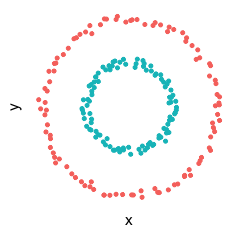
构建一个映射 $\phi: \mathbb{R}^2 \rightarrow \mathbb{R}^3$ 经 $X$ 映射为： $x = x^2, y = y^2, z = y$ ，则通过变换后的数据通过可视化可以明显地看出，数据是可以通过一个超平面来分开的。

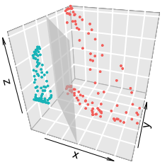
可以说随着维度的增加，我们更有可能找到一个超平面（线性模型）将数据划分开来。尽管看起来，随着维度的增加似乎有助于我们构建模型，但是同时数据在高维空间的分布变得越来越稀疏。因此，在构建机器学习模型时，当我们需要更好的覆盖数据的分布时，我们需要的数据量就更大，这也就会导致需要更多的时间去训练模型。例如，假设所有特征均为0到1之间连续分布的数据，针对1维的情况，当覆盖50%的数据时，仅需全体50%的样本即可；针对2维的情况，当覆盖50%的数据时，则需全体71% ( $0.71^2 \approx 0.5$ ) 的样本；针对3维的情况，当覆盖50%的数据时，则需全体79% ( $0.79^3 \approx 0.5$ )，这就是我们所说的维数灾难。

分散式表示 (Distributed Representations)

分散式表示（Distributed Representations）¹ 最早由 Hiton 提出，对比于传统的 One-Hot Representation ，Distributed Representations 可以将数据表示为低维，稠密，连续的向量，也就是说将原始空间中的潜在信息分散的表示在低维空间的不同维度上。

传统的 One-Hot Representation 会将数据表示成一个很长的向量，例如，在 NLP 中，利用 One-Hot Representation 表示一个单词：

父亲: [1, 0, 0, 0, 0, 0, ...]
爸爸: [0, 1, 0, 0, 0, 0, ...]
母亲: [0, 0, 1, 0, 0, 0, ...]
妈妈: [0, 0, 0, 1, 0, 0, ...]

这种表示形式很简介，但也很稀疏，相当于语料库中有多少个词，则表示空间的维度就需要多少。那么，对于传统的聚类算法，高斯混合模型，最邻近算法，决策树或高斯 SVM 需要 $O\left(N\right)$ 个参数 (或 $O\left(N\right)$ 个样本) 将能够将 $O\left(N\right)$ 的输入区分开来。而像 RBMs ，稀疏编码，Auto-Encoder 或多层神经网络则可以利用 $O\left(N\right)$ 个参数表示 $O\left(2^k\right)$ 的输入，其中 $k \leq N$ 为稀疏表示中非零元素的个数 ²。

采用 Distributed Representation，则可以将单词表示为：

父亲: [0.12, 0.34, 0.65, ...]
爸爸: [0.11, 0.33, 0.58, ...]
母亲: [0.34, 0.98, 0.67, ...]
妈妈: [0.29, 0.92, 0.66, ...]

利用这种表示，我们不仅可以将稀疏的高维空间转换为稠密的低维空间，同时我们还能学习出文本间的语义相似性来，例如实例中的 父亲 和 爸爸，从语义上看其均表示 父亲 的含义，但是如果利用 One-Hot Representation 编码则 父亲 与 爸爸 的距离同其与 母亲 或 妈妈 的距离时相同的，而利用 Distributed Representation 编码，则 父亲 同 爸爸 之间的距离要远小于其同 母亲 或 妈妈 之间的距离。

Word Embedding 之路

N-gram 模型

N-gram (N 元语法) 是一种文本表示方法，指文中连续出现的 $n$ 个词语。N-gram 模型是基于 $n-1$ 阶马尔科夫链的一种概率语言模型，可以通过前 $n-1$ 个词对第 $n$ 个词进行预测。Bengio 等人 ³ 提出了一个三层的神经网络的概率语言模型，其网络结构如下图所示：

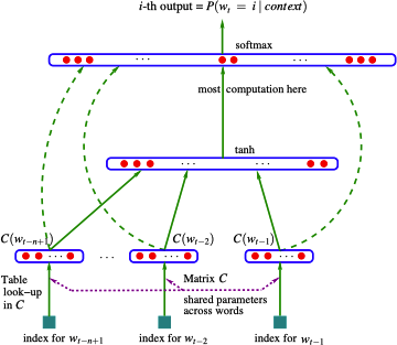
模型的最下面为前 $n-1$ 个词 $w_{t-n+1}, ..., w_{t-2}, w_{t-1}$，每个词 $w_i$ 通过查表的方式同输入层对应的词向量 $C \left(w_i\right)$ 相连。词表 $C$ 为一个 $\lvert V\rvert \times m$ 大小的矩阵，其中 $\lvert V\rvert$ 表示语料中词的数量，$m$ 表示词向量的维度。输入层则为前 $n-1$ 个词向量拼接成的向量 $x$，其维度为 $m \left(n-1\right) \times 1$。隐含层直接利用 $d + Hx$ 计算得到，其中 $H$ 为隐含层的权重，$d$ 为隐含层的偏置。输出层共包含 $\lvert V\rvert$ 个神经元，每个神经元 $y_i$ 表示下一个词为第 $i$ 个词的未归一化的 log 概率，即：

$$ y = b + Wx + U \tanh \left(d + Hx\right) $$

对于该问题，我们的优化目标为最大化如下的 log 似然函数：

$$ L = \dfrac{1}{T} \sum_{t}{f \left(w_t, w_{t-1}, ..., w_{t-n+1}\right) + R \left(\theta\right)} $$

其中，$f \left(w_t, w_{t-1}, ..., w_{t-n+1}\right)$ 为利用前 $n-1$ 个词预测当前词 $w_t$ 的条件概率，$R \left(\theta\right)$ 为参数的正则项，$\theta = \left(b, d, W, U, H, C\right)$。$C$ 作为模型的参数之一，随着模型的训练不断优化，在模型训练完毕后，$C$ 中保存的即为词向量。

Continuous Bag-of-Words (CBOW) 和 Skip-gram 模型

CBOW 和 Skip-gram 均考虑一个词的上下文信息，两种模型的结构如下图所示：

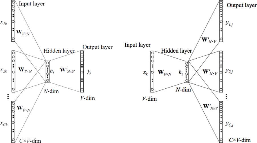
两者在给定的上下文信息中 (即前后各 $m$ 个词) 忽略了上下文环境的序列信息，CBOW (上图左) 是利用上下文环境中的词预测当前的词，而 Skip-gram (上图右) 则是用当前词预测上下文中的词。

对于 CBOW，$x_{1k}, x_{2k}, ..., x_{Ck}$ 为上下文词的 One-Hot 表示，$\mathbf{W}_{V \times N}$ 为所有词向量构成的矩阵 (词汇表)，$y_j$ 为利用上下文信息预测得到的当前词的 One-Hot 表示输出，其中 $C$ 为上下文词汇的数量，$V$ 为词汇表中词的总数量，$N$ 为词向量的维度。从输入层到隐含层，我们对输入层词对应的词向量进行简单的加和，即：

$$ h_i = \sum_{c=1}^{C}{x_{ck} \mathbf{W}_{V \times N}} $$

对于 Skip-gram，$x_k$ 为当前词的 One-Hot 表示，$\mathbf{W}_{V \times N}$ 为所有词向量构成的矩阵 (词汇表)，$y_{1j}, y_{2j}, ..., y_{Cj}$ 为预测的上次文词汇的 One-Hot 表示输出。从输入层到隐含层，直接将 One-Hot 的输入向量转换为词向量表示即可。

除此之外两者还有一些其他的区别：

1. CBOW 要比 Skip-gram 模型训练快。从模型中我们不难发现：从隐含层到输出层，CBOW 仅需要计算一个损失，而 Skip-gram 则需要计算 $C$ 个损失再进行平均进行参数优化。
2. Skip-gram 在小数量的数据集上效果更好，同时对于生僻词的表示效果更好。CBOW 在从输入层到隐含层时，对输入的词向量进行了平均 (可以理解为进行了平滑处理)，因此对于生僻词，平滑后则容易被模型所忽视。

Word2Vec

Mikolov 等人 ⁴ 利用上面介绍的 CBOW 和 Skip-gram 两种模型提出了经典的 Word2Vec 算法。Word2Vec 中针对 CBOW 和 Skip-gram 又提出了两种具体的实现方案 Hierarchical Softmax (层次 Softmax) 和 Negative Sampling (负采样)，因此共有 4 种不同的模型。

• 基于 Hierarchical Softmax 的模型

基于 Hierarchical Softmax 的 CBOW 模型如下：

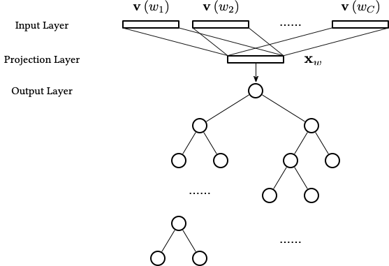
其中：

1. 输入层：包含了 $C$ 个词的词向量，$\mathbf{v} \left(w_1\right), \mathbf{v} \left(w_2\right), ..., \mathbf{v} \left(w_C\right) \in \mathbb{R}^N$，$N$ 为词向量的维度。
2. 投影层：将输入层的向量进行加和，即：$\mathbf{x}_w = \sum_{i=1}^{C}{\mathbf{v} \left(w_i\right)} \in \mathbb{R}^N$。
3. 输出层：输出为一颗二叉树，是根据语料构建出来的 Huffman 树 ⁵，其中每个叶子节点为词汇表中的一个词。

Hierarchical Softmax 是解决概率语言模型中计算效率的关键，CBOW 模型去掉了隐含层，同时将输出层改为了 Huffman 树。对于该模型的优化求解，我们首先引入一些符号，对于 Huffman 树的一个叶子节点 (即词汇表中的词 $w$)，记：

• $p^w$：从根节点出发到达 $w$ 对应的叶子节点的路径。
• $l^w$：路径 $p^w$ 包含的节点的个数。
• $p_1^w, p_1^w, ..., p_{l^w}^w$：路径 $p^w$ 中的 $l^w$ 个节点，其中 $p_1^w$ 表示根节点，$p_{l^w}^w$ 表示词 $w$ 对应的叶子节点。
• $d_2^w, d_3^w, ..., d_{l^w}^w \in \{0, 1\}$：词 $w$ 的 Huffman 编码，由 $l^w - 1$ 位编码构成，$d_j^w$ 表示路径 $p^w$ 中第 $j$ 个结点对应的编码。
• $\theta_1^w, \theta_1^w, ..., \theta_{l^w - 1}^w \in \mathbb{R}^N$：路径 $p^w$ 中非叶子节点对应的向量，$\theta_j^w$ 表示路径 $p^w$ 中第 $j$ 个非叶子节点对应的向量。

首先我们需要根据向量 $\mathbf{x}_w$ 和 Huffman 树定义条件概率 $p \left(w | Context\left(w\right)\right)$。我们可以将其视为一系列的二分类问题，在到达对应的叶子节点的过程中，经过的每一个非叶子节点均为对应一个取值为 0 或 1 的 Huffman 编码。因此，我们可以将编码为 1 的节点定义为负类，将编码为 0 的节点定义为正类 (即分到左边为负类，分到右边为正类)，则这条路径上对应的标签为：

$$ Label \left(p_i^w\right) = 1 - d_i^w, i = 2, 3, ..., l^w $$

则对于一个节点被分为正类的概率为 $\sigma \left(\mathbf{x}_w^{\top} \theta\right)$，被分为负类的概率为 $1 - \sigma \left(\mathbf{x}_w^{\top} \theta\right)$。则条件概率可以表示为：

$$ p \left(w | Context\left(w\right)\right) = \prod_{j=2}^{l^w}{p \left(d_j^w | \mathbf{x}_w, \theta_{j-1}^w\right)} $$

其中

$$ p \left(d_j^w | \mathbf{x}_w, \theta_{j-1}^w\right) = \begin{cases} \sigma \left(\mathbf{x}_w^{\top} \theta\right) & d_j^w = 0 \\ 1 - \sigma \left(\mathbf{x}_w^{\top} \theta\right) & d_j^w = 1 \end{cases} $$

或表示为：

$$ p \left(d_j^w | \mathbf{x}_w, \theta_{j-1}^w\right) = \left[\sigma \left(\mathbf{x}_w^{\top} \theta_{j-1}\right)\right]^{1 - d_j^w} \cdot \left[1 - \sigma \left(\mathbf{x}_w^{\top} \theta_{j-1}\right)\right]^{d_j^w} $$

则对数似然函数为：

$$ \begin{equation} \begin{split} \mathcal{L} &= \sum_{w \in \mathcal{C}}{\log \prod_{j=2}^{l^w}{\left\{\left[\sigma \left(\mathbf{x}_w^{\top} \theta_{j-1}\right)\right]^{1 - d_j^w} \cdot \left[1 - \sigma \left(\mathbf{x}_w^{\top} \theta_{j-1}\right)\right]^{d_j^w}\right\}}} \\ &= \sum_{w \in \mathcal{C}}{\sum_{j=2}^{l^w}{\left\{\left(1 - d_j^w\right) \cdot \log \left[\sigma \left(\mathbf{x}_w^{\top} \theta_{j-1}^w\right)\right] + d_j^w \cdot \log \left[1 - \sigma \left(\mathbf{x}_w^{\top} \theta_{j-1}^w\right)\right]\right\}}} \end{split} \end{equation} $$

记上式花括号中的内容为 $\mathcal{L} \left(w, j\right)$，则 $\mathcal{L} \left(w, j\right)$ 关于 $\theta_{j-1}^w$ 的梯度为：

$$ \begin{equation} \begin{split} \dfrac{\partial \mathcal{L} \left(w, j\right)}{\partial \theta_{j-1}^w} &= \dfrac{\partial}{\partial \theta_{j-1}^w} \left\{\left(1 - d_j^w\right) \cdot \log \left[\sigma \left(\mathbf{x}_w^{\top} \theta_{j-1}^w\right)\right] + d_j^w \cdot \log \left[1 - \sigma \left(\mathbf{x}_w^{\top} \theta_{j-1}^w\right)\right]\right\} \\ &= \left(1 - d_j^w\right) \left[1 - \sigma \left(\mathbf{x}_w^{\top} \theta_{j-1}^w\right)\right] \mathbf{x}_w - d_j^w \sigma \left(\mathbf{x}_w^{\top} \theta_{j-1}^w\right) \mathbf{x}_w \\ &= \left\{\left(1 - d_j^w\right) \left[1 - \sigma \left(\mathbf{x}_w^{\top} \theta_{j-1}^w\right)\right] - d_j^w \sigma \left(\mathbf{x}_w^{\top} \theta_{j-1}^w\right)\right\} \mathbf{x}_w \\ &= \left[1 - d_j^w - \sigma \left(\mathbf{x}_w^{\top} \theta_{j-1}^w\right)\right] \mathbf{x}_w \end{split} \end{equation} $$

则 $\theta_{j-1}^w$ 的更新方式为：

$$ \theta_{j-1}^w \gets \theta_{j-1}^w + \eta \left[1 - d_j^w - \sigma \left(\mathbf{x}_w^{\top} \theta_{j-1}^w\right)\right] \mathbf{x}_w $$

同理可得，$\mathcal{L} \left(w, j\right)$ 关于 $\mathbf{x}_w$ 的梯度为：

$$ \dfrac{\partial \mathcal{L} \left(w, j\right)}{\partial \mathbf{x}_w} = \left[1 - d_j^w - \sigma \left(\mathbf{x}_w^{\top} \theta_{j-1}^w\right)\right] \theta_{j-1}^w $$

但 $\mathbf{x}_w$ 为上下文词汇向量的加和，Word2Vec 的做法是将梯度贡献到上下文中的每个词向量上，即：

$$ \mathbf{v} \left(u\right) \gets \mathbf{v} \left(u\right) + \eta \sum_{j=2}^{l^w}{\dfrac{\partial \mathcal{L} \left(w, j\right)}{\partial \mathbf{x}_w}}, u \in Context \left(w\right) $$

基于 Hierarchical Softmax 的 CBOW 模型的随机梯度上升算法伪代码如下：

    
\begin{algorithm}
\caption{基于 Hierarchical Softmax 的 CBOW 随机梯度上升算法}
\begin{algorithmic}
\STATE $\mathbf{e} = 0$
\STATE $\mathbf{x}_w = \sum_{u \in Context \left(w\right)}{\mathbf{v} \left(u\right)}$
\FOR{$j = 2, 3, ..., l^w$}
    \STATE $q = \sigma \left(\mathbf{x}_w^{\top} \theta_{j-1}^w\right)$
    \STATE $g = \eta \left(1 - d_j^w - q\right)$
    \STATE $\mathbf{e} \gets \mathbf{e} + g \theta_{j-1}^w$
    \STATE $\theta_{j-1}^w \gets \theta_{j-1}^w + g \mathbf{x}_w$
\ENDFOR
\FOR{$u \in Context \left(w\right)$}
    \STATE $\mathbf{v} \left(u\right) \gets \mathbf{v} \left(u\right) + \mathbf{e}$
\ENDFOR
\end{algorithmic}
\end{algorithm}

  

基于 Hierarchical Softmax 的 Skip-gram 模型如下：

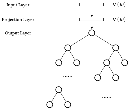
对于 Skip-gram 模型，是利用当前词 $w$ 对上下文 $Context \left(w\right)$ 中的词进行预测，则条件概率为：

$$ p \left(Context \left(w\right) | w\right) = \prod_{u \in Context \left(w\right)}{p \left(u | w\right)} $$

类似于 CBOW 模型的思想，有：

$$ p \left(u | w\right) = \prod_{j=2}^{l^u}{p \left(d_j^u | \mathbf{v} \left(w\right), \theta_{j-1}^u\right)} $$

其中

$$ p \left(d_j^u | \mathbf{v} \left(w\right), \theta_{j-1}^u\right) = \left[\sigma \left(\mathbf{v} \left(w\right)^{\top} \theta_{j-1}^u\right)\right]^{1 - d_j^u} \cdot \left[1 - \sigma \left(\mathbf{v} \left(w\right)^{\top} \theta_{j-1}^u\right)\right]^{d_j^u} $$

可得对数似然函数为：

$$ \begin{equation} \begin{split} \mathcal{L} &= \sum_{w \in \mathcal{C}}{\log \prod_{u \in Context \left(w\right)}{\prod_{j=2}^{l^u}{\left\{\left[\sigma \left(\mathbf{v} \left(w\right)^{\top} \theta_{j-1}^{u}\right)\right]^{1 - d_j^u} \cdot \left[1 - \sigma \left(\mathbf{v} \left(w\right)^{\top} \theta_{j-1}^u\right)\right]^{d_j^u}\right\}}}} \\ &= \sum_{w \in \mathcal{C}}{\sum_{u \in Context \left(w\right)}{\sum_{j=2}^{l^u}{\left\{\left(1 - d_j^u\right) \cdot \log \left[\sigma \left(\mathbf{v} \left(w\right)^{\top} \theta_{j-1}^{u}\right)\right] + d_j^u \cdot \log \left[1 - \sigma \left(\mathbf{v} \left(w\right)^{\top} \theta_{j-1}^{u}\right)\right]\right\}}}} \end{split} \end{equation} $$

记上式花括号中的内容为 $\mathcal{L} \left(w, u, j\right)$，在 $\mathcal{L} \left(w, u, j\right)$ 关于 $\theta_{j-1}^u$ 的梯度为：

$$ \begin{equation} \begin{split} \dfrac{\partial \mathcal{L} \left(w, u, j\right)}{\partial \theta_{j-1}^{u}} &= \dfrac{\partial}{\partial \theta_{j-1}^{u}} \left\{\left(1 - d_j^u\right) \cdot \log \left[\sigma \left(\mathbf{v} \left(w\right)^{\top} \theta_{j-1}^{u}\right)\right] + d_j^u \cdot \log \left[1 - \sigma \left(\mathbf{v} \left(w\right)^{\top} \theta_{j-1}^{u}\right)\right]\right\} \\ &= \left(1 - d_j^u\right) \cdot \left[1 - \sigma \left(\mathbf{v} \left(w\right)^{\top} \theta_{j-1}^{u}\right)\right] \mathbf{v} \left(w\right) - d_j^u \sigma \left(\mathbf{v} \left(w\right)^{\top} \theta_{j-1}^{u}\right) \mathbf{v} \left(w\right) \\ &= \left\{\left(1 - d_j^u\right) \cdot \left[1 - \sigma \left(\mathbf{v} \left(w\right)^{\top} \theta_{j-1}^{u}\right)\right] - d_j^u \sigma \left(\mathbf{v} \left(w\right)^{\top} \theta_{j-1}^{u}\right)\right\} \mathbf{v} \left(w\right) \\ &= \left[1 - d_j^u - \sigma \left(\mathbf{v} \left(w\right)^{\top} \theta_{j-1}^{u}\right)\right] \mathbf{v} \left(w\right) \end{split} \end{equation} $$

则 $\theta_{j-1}^u$ 的更新方式为：

$$ \theta_{j-1}^u \gets \theta_{j-1}^u + \eta \left[1 - d_j^u - \sigma \left(\mathbf{v} \left(w\right)^{\top} \theta_{j-1}^{u}\right)\right] \mathbf{v} \left(w\right) $$

同理可得，$\mathcal{L} \left(w, u, j\right)$ 关于 $\mathbf{v} \left(w\right)$ 的梯度为：

$$ \dfrac{\partial \mathcal{L} \left(w, u, j\right)}{\partial \mathbf{v} \left(w\right)} = \left[1 - d_j^u - \sigma \left(\mathbf{v} \left(w\right)^{\top} \theta_{j-1}^{u}\right)\right] \theta_{j-1}^u $$

则 $\mathbf{v} \left(w\right)$ 的更新方式为：

$$ \mathbf{v} \left(w\right) \gets \mathbf{v} \left(w\right) + \eta \sum_{u \in Context \left(w\right)}{\sum_{j=2}^{l^u}{\dfrac{\partial \mathcal{L} \left(w, u, j\right)}{\partial \mathbf{v} \left(w\right)}}} $$

基于 Hierarchical Softmax 的 Skip-gram 模型的随机梯度上升算法伪代码如下：

    
\begin{algorithm}
\caption{基于 Hierarchical Softmax 的 Skig-gram 随机梯度上升算法}
\begin{algorithmic}
\STATE $\mathbf{e} = 0$
\FOR{$u \in Context \left(w\right)$}
    \FOR{$j = 2, 3, ..., l^u$}
        \STATE $q = \sigma \left(\mathbf{x}_w^{\top} \theta_{j-1}^u\right)$
        \STATE $g = \eta \left(1 - d_j^u - q\right)$
        \STATE $\mathbf{e} \gets \mathbf{e} + g \theta_{j-1}^u$
        \STATE $\theta_{j-1}^u \gets \theta_{j-1}^u + g \mathbf{v} \left(w\right)$
    \ENDFOR
\ENDFOR
\STATE $\mathbf{v} \left(w\right) \gets \mathbf{v} \left(w\right) + \mathbf{e}$
\end{algorithmic}
\end{algorithm}

  

• 基于 Negative Sampling 的模型

基于 Negative Sampling (NEG) 的模型相比于基于 Hierarchical Softmax 的模型不再使用复杂的 Huffman 树，而是使用简单的随机负采样，从而大幅的提高了模型的性能。

基于 Negative Sampling 的 CBOW 模型如下：

对于基于 Negative Sampling CBOW 模型，已知词 $w$ 的上下文 $Context \left(w\right)$，预测词 $w$，则词 $w$ 即为一个正样本，其他词则为负样本。对于一个给定 $Context \left(w\right)$ 的负样本集合 $NEG \left(w\right) \neq \varnothing$，词典中的任意词 $\forall \tilde{w} \in \mathcal{D}$，其样本的标签定义为：

$$ L^w \left(\tilde{w}\right) = \begin{cases} 1, & \tilde{w} = w \\ 0, & \tilde{w} \neq w \end{cases} $$

则对于一个正样本 $\left(Context, \left(w\right)\right)$，我们希望最大化：

$$ g \left(w\right) = \prod_{u \in \left\{w\right\} \cup NEG \left(w\right)}{p \left(u | Context \left(w\right)\right)} $$

或表示为：

$$ p \left(u | Context \left(w\right)\right) = \left[\sigma \left(\mathbf{x}_w^{\top} \theta^u\right)\right]^{L^w \left(w\right)} \cdot \left[1 - \sigma \left(\mathbf{x}_w^{\top} \theta^u\right)\right]^{1 - L^w \left(w\right)} $$

即增大正样本概率的同时减少负样本的概率。对于一个给定的语料库 $\mathcal{C}$，对数似然函数为：

$$ \begin{equation} \begin{split} \mathcal{L} &= \sum_{w \in \mathcal{C}}{\log g \left(w\right)} \\ &= \sum_{w \in \mathcal{C}}{\log \prod_{u \in \left\{w\right\} \cup NEG \left(w\right)}{\left\{\left[\sigma \left(\mathbf{x}_w^{\top} \theta^u\right)\right]^{L^w \left(u\right)} \cdot \left[1 - \sigma \left(\mathbf{x}_w^{\top} \theta^u\right)\right]^{1 - L^w \left(u\right)}\right\}}} \\ &= \sum_{w \in \mathcal{C}}{\sum_{u \in \left\{w\right\} \cup NEG \left(w\right)}{\left\{L^w \left(u\right) \cdot \log \left[\sigma \left(\mathbf{x}_w^{\top} \theta^u\right)\right] + \left[1 - L^w \left(u\right)\right] \cdot \log \left[1 - \sigma \left(\mathbf{x}_w^{\top} \theta^u\right)\right]\right\}}} \end{split} \end{equation} $$

记上式花括号中的内容为 $\mathcal{L} \left(w, u\right)$，则 $\mathcal{L} \left(w, u\right)$ 关于 $\theta^u$ 的梯度为：

$$ \begin{equation} \begin{split} \dfrac{\partial \mathcal{L} \left(w, u\right)}{\partial \theta^u} &= \dfrac{\partial}{\partial \theta^u} \left\{L^w \left(u\right) \cdot \log \left[\sigma \left(\mathbf{x}_w^{\top} \theta^u\right)\right] + \left[1 - L^w \left(u\right)\right] \cdot \log \left[1 - \sigma \left(\mathbf{x}_w^{\top} \theta^u\right)\right]\right\} \\ &= L^w \left(u\right) \left[1 - \sigma \left(\mathbf{w}_w^{\top} \theta^u\right)\right] \mathbf{x}_w - \left[1 - L^w \left(u\right)\right] \sigma \left(\mathbf{x}_w^{\top} \theta^u\right) \mathbf{x}_w \\ &= \left\{L^w \left(u\right) \left[1 - \sigma \left(\mathbf{w}_w^{\top} \theta^u\right)\right] - \left[1 - L^w \left(u\right)\right] \sigma \left(\mathbf{x}_w^{\top} \theta^u\right)\right\} \mathbf{x}_w \\ &= \left[L^w \left(u\right) - \sigma \left(\mathbf{w}_w^{\top} \theta^u\right)\right] \mathbf{x}_w \end{split} \end{equation} $$

则 $\theta^u$ 的更新方式为：

$$ \theta^u \gets \theta^u + \eta \left[L^w \left(u\right) - \sigma \left(\mathbf{w}_w^{\top} \theta^u\right)\right] \mathbf{x}_w $$

同理可得，$\mathcal{L} \left(w, u\right)$ 关于 $\mathbf{x}_w$ 的梯度为：

$$ \dfrac{\partial \mathcal{L} \left(w, u\right)}{\partial \mathbf{x}_w} = \left[L^w \left(u\right) - \sigma \left(\mathbf{w}_w^{\top} \theta^u\right)\right] \theta^u $$

则 $\mathbf{v} \left(\tilde{w}\right), \tilde{w} \in Context \left(w\right)$ 的更新方式为：

$$ \mathbf{v} \left(\tilde{w}\right) \gets \mathbf{v} \left(\tilde{w}\right) + \eta \sum_{u \in \left\{w\right\} \cup NEG \left(w\right)}{\dfrac{\partial \mathcal{L} \left(w, u\right)}{\partial \mathbf{x}_w}}, \tilde{w} \in Context \left(w\right) $$

基于 Negative Sampling 的 CBOW 模型的随机梯度上升算法伪代码如下：

    
\begin{algorithm}
\caption{基于 Negative Sampling 的 CBOW 随机梯度上升算法}
\begin{algorithmic}
\STATE $\mathbf{e} = 0$
\STATE $\mathbf{x}_w = \sum_{u \in Context \left(w\right)}{\mathbf{v} \left(u\right)}$
\FOR{$u \in Context \left\{w\right\} \cup NEG \left(w\right)$}
    \STATE $q = \sigma \left(\mathbf{x}_w^{\top} \theta^u\right)$
    \STATE $g = \eta \left(L^w \left(u\right) - q\right)$
    \STATE $\mathbf{e} \gets \mathbf{e} + g \theta^u$
    \STATE $\theta^u \gets \theta^u + g \mathbf{x}_w$
\ENDFOR
\FOR{$u \in Context \left(w\right)$}
    \STATE $\mathbf{v} \left(u\right) \gets \mathbf{v} \left(u\right) + \mathbf{e}$
\ENDFOR
\end{algorithmic}
\end{algorithm}

  

基于 Negative Sampling 的 Skip-gram 模型如下：

对于 Skip-gram 模型，利用当前词 $w$ 对上下文 $Context \left(w\right)$ 中的词进行预测，则对于一个正样本 $\left(Context, \left(w\right)\right)$，我们希望最大化：

$$ g \left(w\right) = \prod_{\tilde{w} \in Context \left(w\right)}{\prod_{u \in \left\{w\right\} \cup NEG^{\tilde{w}} \left(w\right)}{p \left(u | \tilde{w}\right)}} $$

其中，$NEG^{\tilde{w}} \left(w\right)$ 为处理词 $\tilde{w}$ 时生成的负样本集合，且：

$$ p \left(u | \tilde{w}\right) = \begin{cases} \sigma \left(\mathbf{v}\left(\tilde{w}\right)^{\top} \theta^u\right) & L^w \left(u\right) = 1 \\ 1 - \sigma \left(\mathbf{v}\left(\tilde{w}\right)^{\top} \theta^u\right) & L^w \left(u\right) = 0 \end{cases} $$

或表示为：

$$ p \left(u | \tilde{w}\right) = \left[\sigma \left(\mathbf{v}\left(\tilde{w}\right)^{\top} \theta^u\right)\right]^{L^w \left(u\right)} \cdot \left[1 - \sigma \left(\mathbf{v}\left(\tilde{w}\right)^{\top} \theta^u\right)\right]^{1 - L^w \left(u\right)} $$

对于一个给定的语料库 $\mathcal{C}$，对数似然函数为：

$$ \begin{equation} \begin{split} \mathcal{L} &= \sum_{w \in \mathcal{C}}{\log g \left(w\right)} \\ &= \sum_{w \in \mathcal{C}}{\log \prod_{\tilde{w} \in Context \left(w\right)}{\prod_{u \in \left\{w\right\} \cup NEG^{\tilde{w}} \left(w\right)}{\left\{\left[\sigma \left(\mathbf{v}\left(\tilde{w}\right)^{\top} \theta^u\right)\right]^{L^w \left(u\right)} \cdot \left[1 - \sigma \left(\mathbf{v}\left(\tilde{w}\right)^{\top} \theta^u\right)\right]^{1 - L^w \left(u\right)}\right\}}}} \\ &= \sum_{w \in \mathcal{C}}{\sum_{\tilde{w} \in Context \left(w\right)}{\sum_{u \in \left\{w\right\} \cup NEG^{\tilde{w}} \left(w\right)}{\left\{L^w \left(u\right) \cdot \log \left[\sigma \left(\mathbf{v}\left(\tilde{w}\right)^{\top} \theta^u\right)\right] + \left[1 - L^w \left(u\right)\right] \cdot \log \left[1 - \sigma \left(\mathbf{v}\left(\tilde{w}\right)^{\top} \theta^u\right)\right]\right\}}}} \end{split} \end{equation} $$

记上式花括号中的内容为 $\mathcal{L} \left(w, \tilde{w}, u\right)$，则 $\mathcal{L} \left(w, \tilde{w}, u\right)$ 关于 $\theta^u$ 的梯度为：

$$ \begin{equation} \begin{split} \dfrac{\partial \mathcal{L} \left(w, \tilde{w}, u\right)}{\partial \theta^u} &= \dfrac{\partial}{\partial \theta^u} \left\{L^w \left(u\right) \cdot \log \left[\sigma \left(\mathbf{v}\left(\tilde{w}\right)^{\top} \theta^u\right)\right] + \left[1 - L^w \left(u\right)\right] \cdot \log \left[1 - \sigma \left(\mathbf{v}\left(\tilde{w}\right)^{\top} \theta^u\right)\right]\right\} \\ &= L^w \left(u\right) \left[1 - \sigma \left(\mathbf{v} \left(\tilde{w}\right)^{\top} \theta^u\right)\right] \mathbf{v} \left(\tilde{w}\right) - \left[1 - L^w \left(u\right)\right] \sigma \left(\mathbf{v} \left(\tilde{w}\right)^{\top} \theta^u\right) \mathbf{v} \left(\tilde{w}\right) \\ &= \left\{L^w \left(u\right) \left[1 - \sigma \left(\mathbf{v} \left(\tilde{w}\right)^{\top} \theta^u\right)\right] - \left[1 - L^w \left(u\right)\right] \sigma \left(\mathbf{v} \left(\tilde{w}\right)^{\top} \theta^u\right)\right\} \mathbf{v} \left(\tilde{w}\right) \\ &= \left[L^w \left(u\right) - \sigma \left(\mathbf{v} \left(\tilde{w}\right)^{\top} \theta^u\right)\right] \mathbf{v} \left(\tilde{w}\right) \end{split} \end{equation} $$

则 $\theta^u$ 的更新方式为：

$$ \theta^u \gets \theta^u + \eta \left[L^w \left(u\right) - \sigma \left(\mathbf{v} \left(\tilde{w}\right)^{\top} \theta^u\right)\right] \mathbf{v} \left(\tilde{w}\right) $$

同理可得，$\mathcal{L} \left(w, \tilde{w}, u\right)$ 关于 $\mathbf{v} \left(\tilde{w}\right)$ 的梯度为：

$$ \dfrac{\partial \mathcal{L} \left(w, \tilde{w}, u\right)}{\partial \mathbf{v} \left(\tilde{w}\right)} = \left[L^w \left(u\right) - \sigma \left(\mathbf{v} \left(\tilde{w}\right)^{\top} \theta^u\right)\right] \theta^u $$

则 $\mathbf{v} \left(\tilde{w}\right)$ 的更新方式为：

$$ \mathbf{v} \left(\tilde{w}\right) \gets \mathbf{v} \left(\tilde{w}\right) + \eta \sum_{u \in \left\{w\right\} \cup NEG^{\tilde{w}} \left(w\right)}{\dfrac{\partial \mathcal{L} \left(w, \tilde{w}, u\right)}{\partial \mathbf{v} \left(\tilde{w}\right)}} $$

基于 Negative Sampling 的 Skig-gram 模型的随机梯度上升算法伪代码如下：

    
\begin{algorithm}
\caption{基于 Negative Sampling 的 Skig-gram 随机梯度上升算法}
\begin{algorithmic}
\STATE $\mathbf{e} = 0$
\FOR{$\tilde{w} \in Context \left(w\right)$}
    \FOR{$u \in \left\{w\right\} \cup NEG^{\tilde{w}} \left(w\right)$}
        \STATE $q = \sigma \left(\mathbf{v} \left(\tilde{w}\right)^{\top} \theta^u\right)$
        \STATE $g = \eta \left(L^w \left(u\right) - q\right)$
        \STATE $\mathbf{e} \gets \mathbf{e} + g \theta^u$
        \STATE $\theta^u \gets \theta^u + g \mathbf{v} \left(\tilde{w}\right)$
    \ENDFOR
\ENDFOR
\STATE $\mathbf{v} \left(\tilde{w}\right) \gets \mathbf{v} \left(\tilde{w}\right) + \mathbf{e}$
\end{algorithmic}
\end{algorithm}

  

无论是基于 Negative Sampling 的 CBOW 模型还是 Skip-gram 模型，我们都需要对于给定的词 $w$ 生成 $NEG \left(w\right)$，对于一个词典 $\mathcal{D}$ 和给定的语料 $\mathcal{C}$，一个词被选择中的概率为：

$$ p_{NEG} \left(w\right) = \dfrac{\#w}{\sum_{u \in \mathcal{D}}{\#u}} $$

其中 $\#w$ 和 $\#u$ 表示词 $w$ 和 $u$ 在语料 $\mathcal{C}$ 中出现的频次。在 Word2Vec 的 C 代码中 ⁶，并没有使用词的原始频次，而是对其做了 0.75 次幂，即：

$$ p_{NEG} \left(w\right) = \dfrac{\left(\#w\right)^{0.75}}{\sum_{u \in \mathcal{D}}{\left(\#u\right)^{0.75}}} $$

其他 Embedding 方法

GloVe

GloVe (Global Vector 的简写) 是由 Pennington 等人 ⁷ 提出了一种词向量生成方法，该方法利用了语料的全局统计信息。

令 $X$ 表示词与词之间的共现矩阵，$X_{ij}$ 表示词 $j$ 在词 $i$ 为上下文的情况下出现的频次。则 $X_i = \sum_{k}{X_{ik}}$ 表示在词$i$ 为上下文的情况任意词出现的总次数。令 $P_{ij} = P \left(j | i\right) = X_{ij} / X_i$ 表示词 $j$ 在词 $i$ 出现前提下出现的条件概率。

例如，我们令 $i = ice, j = steam$，则这两个词之间的关系可以利用同其他词 $k$ 共现概率的比率学习得出。则有：

1. 与词 ice 相关，但与词 steam 不太相关，例如 $k = solid$，则比率 $P_{ik} / P_{jk}$ 应该较大；类似的当词 $k$ 与 steam 相关，但与词 ice 不太相关，则比率 $P_{ik} / P_{jk}$ 应该较小。
2. 当与词 ice 和词 steam 均相关或者均不太相关时，例如 $k = water$ 或 $k = fashion$，则比率 $P_{ik} / P_{jk}$ 应该和 1 接近。

下表展示了在一个大量语料上的概率及其比率：

根据如上的假设，我们可以得到一个最基础的模型：

$$ F \left(w_i, w_j, \tilde{w}_k\right) = \dfrac{P_{ik}}{P_{jk}} $$

其中 $w \in \mathbb{R}^d$ 为词向量，$\tilde{w}_k \in \mathbb{R}^d$ 为单独的上下文词的词向量。假设向量空间是一个线性结构，因此 $F$ 仅依赖于两个向量之间的差异，则模型可以改写为：

$$ F \left(w_i - w_j, \tilde{w}_k\right) = \dfrac{P_{ik}}{P_{jk}} $$

上式中右面是一个标量，如果左面的参数利用一个复杂的模型进行计算，例如神经网络，则会破坏我们希望保留的线性结构。因此，我们对参数采用点积运算，即：

$$ F \left(\left(w_i - w_j\right)^{\top} \tilde{w}_k\right) = \dfrac{P_{ik}}{P_{jk}} $$

在词之间的共现矩阵中，一个词和其上下文中的一个词之间应该是可以互换角色的。首先我们要保证 $F$ 在 $\left(\mathbb{R}, +\right)$ 和 $\left(\mathbb{R}_{>0}, \times\right)$ 上是同态的 (homomorphism)，例如：

$$ F \left(\left(w_i - w_j\right)^{\top} \tilde{w}_k\right) = \dfrac{F \left(w_i^{\top} \tilde{w}_k\right)}{F \left(w_j^{\top} \tilde{w}_k\right)} $$

其中 $F \left(w_i^{\top} \tilde{w}_k\right) = P_{ik} = \dfrac{X_{ik}}{X_i}$，则上式的一个解为 $F = \exp$，或：

$$ w_i^{\top} \tilde{w}_k = \log \left(P_{ik}\right) = \log \left(X_{ik}\right) - \log \left(X_i\right) $$

其中 $\log \left(X_i\right)$ 与 $k$ 无关记为 $b_i$，同时为了对称性添加 $\tilde{b}_k$，则上式改写为：

$$ w_i^{\top} \tilde{w}_k + b_i + \tilde{b}_k = \log \left(X_{ik}\right) $$

上式中，左侧为词向量的相关运算，右侧为共现矩阵的常量信息，则给出模型的损失函数如下：

$$ J = \sum_{i,j=1}^{V}{f \left(X_{ij}\right) \left(w_i^{\top} \tilde{w}_k + b_i + \tilde{b}_k - \log X_{ij}\right)^2} $$

其中，$V$ 为词典中词的个数，$f$ 为一个权重函数，其应具有如下特点：

1. $f \left(0\right) = 0$。如果 $f$ 为一个连续函数，则当 $x \to 0$ 时 $\lim_{x \to 0}{f \left(x\right) \log^2 x}$ 应足够快地趋近于无穷。
2. $f \left(x\right)$ 应为非减函数，以确保稀少的共现不会权重过大。
3. $f \left(x\right)$ 对于较大的 $x$ 应该相对较小，以确保过大的共现不会权重过大。

文中给出了一个符合要求的函数如下：

$$ f \left(x\right) = \begin{cases} \left(x / x_{\max}\right)^{\alpha} & \text{if} \ x < x_{\max} \\ 1 & \text{otherwise} \end{cases} $$

其中两个超参数的值建议为 $x_{\max} = 100, \alpha = 0.75$。

fastText

fastText 是由 Bojanowski 和 Grave 等人 ⁸ 提出的一种词向量表示方法。原始的 Skip-gram 模型忽略了词语内部的结构信息，fastText 利用 N-gram 方法将其考虑在内。

对于一个词 $w$，利用一系列的 N-gram 进行表示，同时在词的前后添加 < 和 > 边界符号以同其他文本序列进行区分。同时还将词语本身也包含在这个 N-gram 集合中，从而学习到词语的向量表示。例如，对于词 $where$ 和 $n = 3$，则 N-gram 集合为：<wh, whe, her, ere, re>，同时包含词本身 <where>。需要注意的是，序列 <her> 与词 $where$ 中的 tri-gram her 是两个不同的概念。模型提取所有 $3 \leq n \leq 6$ 的 N-gram 序列。

假设 N-gram 词典的大小为 $G$，对于一个词 $w$，$\mathcal{G}_w \subset \left\{1, ..., G\right\}$ 表示词中出现的 N-gram 的集合。针对任意一个 N-gram $g$，用向量 $\mathbf{z}_g$ 表示，则我们利用一个词的所有 N-gram 的向量的加和表示该词。可以得到该模型的评分函数为：

$$ s \left(w, c\right) = \sum_{g \in \mathcal{G}_w}{\mathbf{z}_g^{\top} \mathbf{v}_c} $$

模型在学习不同词向量时可以共享权重 (不同词的可能包含相同的 N-gram)，使得在学习低频词时也可得到可靠的向量表示。

WordRank

WordRank 是由 Ji 等人 ⁹ 提出的一种词向量表示方法，其将词向量学习问题转换成一个排序问题。

我们令 $\mathbf{u}_w$ 表示当前词 $w$ 的 $k$ 维词向量，$\mathbf{v}_c$ 表示当前词上下文 $c$ 的词向量。通过两者的内积 $\langle \mathbf{u}_w, \mathbf{v}_c \rangle$ 来捕获词 $w$ 和上下文 $c$ 之间的关系，两者越相关则该内积越大。对于一个给定的词 $w$，利用上下文集合 $\mathcal{C}$ 同词的内积分数进行排序，对于一个给定的上下文 $c$，排序为：

$$ \begin{equation} \begin{split} \text{rank} \left(w, c\right) &= \sum_{c' \in \mathcal{C} \setminus \left\{c\right\}}{I \left(\langle \mathbf{u}_w, \mathbf{v}_c \rangle - \langle \mathbf{u}_w, \mathbf{v}_{c'} \rangle \leq 0\right)} \\ &= \sum_{c' \in \mathcal{C} \setminus \left\{c\right\}}{I \left(\langle \mathbf{u}_w, \mathbf{v}_c - \mathbf{v}_{c'} \rangle \leq 0\right)} \end{split} \end{equation} $$

其中，$I \left(x \leq 0\right)$ 为一个 0-1 损失函数，当 $x \leq 0$ 时为 1 其他情况为 0。由于 $I \left(x \leq 0\right)$ 为一个非连续函数，因此我们可以将其替换为一个凸上限函数 $\ell \left(\cdot\right)$，其可以为任意的二分类损失函数，构建排序的凸上限如下：

$$ \text{rank} \left(w, c\right) \leq \overline{\text{rank}} \left(w, c\right) = \sum_{c' \in \mathcal{C} \setminus \left\{c\right\}}{\ell \left(\langle \mathbf{u}_w, \mathbf{v}_c - \mathbf{v}_{c'} \rangle\right)} $$

我们期望排序模型将更相关的上下文排在列表的顶部，基于此构建损失函数如下：

$$ J \left(\mathbf{U}, \mathbf{V}\right) := \sum_{w \in \mathcal{W}}{\sum_{c \in \Omega_w}{r_{w, c} \cdot \rho \left(\dfrac{\overline{\text{rank}} \left(w, c\right) + \beta}{\alpha}\right)}} $$

其中，$\mathcal{W}$ 表示词典，$\mathbf{U} := \left\{\mathbf{u}_w\right\}_{w \in \mathcal{W}}$ 和 $\mathbf{V} := \left\{\mathbf{c}_w\right\}_{c \in \mathcal{C}}$ 分别表示词及其上下文词向量的参数，$\Omega_w$ 表示与词 $w$ 共现的上下文的集合，$r_{w, c}$ 为衡量 $w$ 和 $c$ 之间关系的权重，$\rho \left(\cdot\right)$ 为用于衡量排序好坏的单调递增的损失函数，$\alpha \geq 0, \beta \geq 0$ 为超参数。可选的有：

$$ r_{w, c} = \begin{cases} \left(X_{w, c} / x_{\max}\right)^{\epsilon} & \text{if} \ X_{w, c} < x_{\max} \\ 1 & \text{otherwise} \end{cases} $$

其中 $x_{\max} = 100, \epsilon = 0.75$。根据 $\rho \left(\cdot\right)$ 的要求，损失函数在排序的顶部 (rank 值小) 的地方更加敏感，同时对于 rank 值较大的地方不敏感。这可以使得模型变得更加稳健 (避免语法错误和语言的非常规使用造成干扰)，因此可选的有：

$$ \begin{equation} \begin{split} \rho \left(x\right) &:= \log_2 \left(1 + x\right) \\ \rho \left(x\right) &:= 1 - \dfrac{1}{\log_2 \left(2 + x\right)} \\ \rho \left(x\right) &:= \dfrac{x^{1 - t} - 1}{1 - t}, t \neq 1 \end{split} \end{equation} $$

损失函数可以等价的定义为：

$$ J \left(\mathbf{U}, \mathbf{V}\right) := \sum_{\left(w, c\right) \in \Omega}{r_{w, c} \cdot \rho \left(\dfrac{\overline{\text{rank}} \left(w, c\right) + \beta}{\alpha}\right)} $$

在训练过程中，外层的求和符号容易利用 SDG 算法解决，但对于内层的求和符号除非 $\rho \left(\cdot\right)$ 是一个线性函数，否则难以求解。然而，$\rho \left(\cdot\right)$ 函数的性质要求其不能是一个线性函数，但我们可以利用其凹函数的特性对其进行一阶泰勒分解，有：

$$ \rho \left(x\right) \leq \rho \left(\xi^{-1}\right) + \rho' \left(\xi^{-1}\right) \cdot \left(x - \xi^{-1}\right) $$

对于任意 $x$ 和 $\xi \neq 0$ 均成立，同时当且仅当 $\xi = x^{-1}$ 时等号成立。因此，令 $\Xi := \left\{\xi_{w, c}\right\}_{\left(w, c\right) \in \Sigma}$，则可以得到 $J \left(\mathbf{U}, \mathbf{V}\right)$ 的一个上界：

$$ \begin{equation} \begin{split} \overline{J} \left(\mathbf{U}, \mathbf{V}, \Xi\right) &:= \sum_{\left(w, c\right) \in \Omega}{r_{w, c} \cdot \left\{\rho \left(\xi_{wc}^{-1}\right) + \rho' \left(\xi_{wc}^{-1}\right) \cdot \left(\alpha^{-1} \beta + \alpha^{-1} \sum_{c' \in \mathcal{C} \setminus \left\{c\right\}}{\ell \left(\langle \mathbf{u}_w, \mathbf{v}_c - \mathbf{v}_{c'} \rangle\right) - \xi_{w, c}^{-1}}\right)\right\}} \\ &= \sum_{\left(w, c, c'\right)}{r_{w, c} \cdot \left(\dfrac{\rho \left(\xi_{w, c}^{-1}\right) + \rho' \left(\xi_{w, c}^{-1}\right) \cdot \left(\alpha^{-1} \beta - \xi_{w, c}^{-1}\right)}{\lvert \mathcal{C} \rvert - 1} + \dfrac{1}{\alpha} \rho' \left(\xi_{w, c}^{-1}\right) \cdot \ell \left(\langle \mathbf{u}_w, \mathbf{v}_c - \mathbf{v}_{c'} \rangle\right)\right)} \end{split} \end{equation} $$

其中，$\left(w, c, c'\right) \in \Omega \times \left(\mathcal{C} \setminus \left\{c\right\}\right)$，至此我们可以通过均匀采样 $\left(w, c\right) \in \Sigma$ 和 $c' \in \mathcal{C} \setminus \left\{c\right\}$ 解决训练问题。

整个 WordRank 算法的伪代码如下：

    
\begin{algorithm}
\caption{WordRank 算法}
\begin{algorithmic}
\STATE $\eta$ 为学习率
\WHILE{$\mathbf{U}$，$\mathbf{V}$ 和 $\Xi$ 未收敛}
    \STATE \COMMENT{阶段1：更新 $\mathbf{U}$ 和 $\mathbf{V}$}
    \WHILE{$\mathbf{U}$ 和 $\mathbf{V}$ 未收敛}
        \STATE 从 $\Omega$ 中均匀采样 $\left(w, c\right)$
        \STATE 从 $\mathcal{C} \setminus \left\{c\right\}$ 中均匀采样 $c'$
        \STATE \COMMENT{同时更新如下 3 个参数}
        \STATE $\mathbf{u}_w \gets \mathbf{u}_w - \eta \cdot r_{w, c} \cdot \rho' \left(\xi_{w, c}^{-1}\right) \cdot \ell' \left(\langle \mathbf{u}_w, \mathbf{v}_c - \mathbf{v}_{c'} \rangle\right) \cdot \left(\mathbf{v}_c - \mathbf{v}_{c'}\right)$
        \STATE $\mathbf{v}_c \gets \mathbf{v}_c - \eta \cdot r_{w, c} \cdot \rho' \left(\xi_{w, c}^{-1}\right) \cdot \ell' \left(\langle \mathbf{u}_w, \mathbf{v}_c - \mathbf{v}_{c'} \rangle\right) \cdot \mathbf{u}_w$
        \STATE $\mathbf{v}_{c'} \gets \mathbf{v}_{c'} - \eta \cdot r_{w, c} \cdot \rho' \left(\xi_{w, c}^{-1}\right) \cdot \ell' \left(\langle \mathbf{u}_w, \mathbf{v}_c - \mathbf{v}_{c'} \rangle\right) \cdot \mathbf{u}_w$
    \ENDWHILE
    \STATE \COMMENT{阶段2：更新 $\Xi$}
    \FOR{$w \in \mathcal{W}$}
        \FOR{$c \in \mathcal{C}$}
            \STATE $\xi_{w, c} = \alpha / \left(\sum_{c' \in \mathcal{C} \setminus \left\{c\right\}}{\ell \left(\langle \mathbf{u}_w, \mathbf{v}_c - \mathbf{v}_{c'} \rangle\right) + \beta}\right)$
        \ENDFOR
    \ENDFOR
\ENDWHILE
\end{algorithmic}
\end{algorithm}

  

cw2vec

cw2vec 是由 Cao 等人 ¹⁰ 提出的一种基于汉字笔画 N-gram 的中文词向量表示方法。该方法根据汉字作为象形文字具有笔画信息的特点，提出了笔画 N-gram 的概念。针对一个词的笔画 N-gram，其生成过程如下图所示：

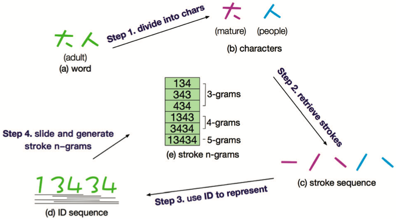
共包含 4 个步骤：

1. 将一个词拆解成单个的汉字，例如：“大人” 拆解为 “大” 和 “人”。
2. 将每个汉字拆解成笔画，例如：“大” 和 “人” 拆解为 “一，丿，乀，丿，乀”。
3. 将每个笔画映射到对应的编码序列，例如： “一，丿，乀，丿，乀” 映射为 13434。
4. 利用编码序列生成笔画 N-gram，例如：134，343，434；1343，3434；13434。

模型中定义一个词 $w$ 及其上下文 $c$ 的相似度如下：

$$ sim \left(w, c\right) = \sum_{q \in S\left(w\right)}{\vec{q} \cdot \vec{c}} $$

其中，$S$ 为由笔画 N-gram 构成的词典，$S \left(w\right)$ 为词 $w$ 对应的笔画 N-gram 集合，$q$ 为该集合中的一个笔画 N-gram，$\vec{q}$ 为 $q$ 对应的向量。

该模型的损失函数为：

$$ \mathcal{L} = \sum_{w \in D}{\sum_{c \in T \left(w\right)}{\log \sigma \left(sim \left(w, c\right)\right) + \lambda \mathbb{E}_{c' \sim P} \left[\log \sigma \left(- sim \left(w, c'\right)\right)\right]}} $$

其中，$D$ 为语料中的全部词语，$T \left(w\right)$ 为给定的词 $w$ 和窗口内的所有上次文词，$\sigma \left(x\right) = \left(1 + \exp \left(-x\right)\right)^{-1}$，$\lambda$ 为负采样的个数，$\mathbb{E}_{c' \sim P} \left[\cdot\right]$ 表示负样本 $c'$ 按照 $D$ 中词的分布 $P$ 进行采样，该分布可以为词的一元模型的分布 $U$，同时为了避免数据的稀疏性问题，类似 Word2Vec 中的做法采用 $U^{0.75}$。