• Pruning helps reduce LLM inference cost by lowering the number of non-zero weights and reducing memory pressure.
• SparseGPT is stronger for quality retention, especially when pruning aggressively or targeting higher sparsity levels.
• Wanda is faster and easier to implement because it avoids Hessian estimation, reconstruction solving, and weight updates.
• Sparse models are not automatically faster; real speedups require sparse-aware runtimes, sparse kernels, and hardware support.
• Pruning works best as part of a larger inference optimization strategy, combined with quantization, KV-cache optimization, batching, caching, speculative decoding, and routing.

LLM inference is constrained by four major production bottlenecks:

• GPU VRAM capacity. Model weights, KV cache, runtime tensors, and multiple in-flight requests must all fit in memory. Offline testing may show the model is “functional,” but under real traffic conditions, it may fail due to memory pressure from increased active sequence lengths and batch sizes.
• Memory bandwidth. During autoregressive decoding, the model emits one token at a time. To emit each token, the GPU must repeatedly load model weights and cached attention states. This often makes decoding memory-bound instead of compute-bound. In that case, a GPU with more raw FLOPs does not always deliver proportional speedups.
• Latency. Real user-facing apps require low time-to-first-token, consistent inter-token latency, and predictable end-to-end latency. You could have a model that generates high-quality answers, but if the responses are slow, the user experience suffers.
• Cost. GPU cloud infrastructure is expensive when GPUs are underutilized, overprovisioned, or blocked by memory limits. At scale, even small efficiency improvements can reduce cost per million tokens.

Pruning reduces the total number of non‑zero weights in the model. Sparse models store many zeros. In theory, this reduces memory and compute needs. If the inference stack can take advantage of this sparsity—using compressed storage formats and sparse matrix multiplication kernels—models can achieve lower VRAM footprint, higher throughput, and reduced latency. Real-world speedups depend on the hardware and software used to run the model. Zeroing weights without changing the kernel will not speed up inference.

Beyond GPU servers, compression enables new modes of deployment. Pruned models can be deployed to smaller GPUs, edge devices, or even multi‑model servers. Memory savings let teams colocate several models on a single GPU, use cheaper instances, or fit larger batch sizes for the same hardware budget. Compression is directly tied to the economics of inference: reducing memory per token reduces the cost per token.

Neural networks are typically dense, meaning that most of their weights are non-zero. A sparse network, on the other hand, consists mostly of zero-valued weights. Network pruning increases sparsity by permanently setting weights to zero. For language models, there are two particularly important types of sparsity: unstructured and structured.

Unstructured sparsity

Unstructured pruning removes individual weights at random throughout the model.This allows the pruning algorithm maximum flexibility in choosing which weights to remove while minimizing impact on model behavior. Because weights can be removed from the matrix at any position, unstructured sparsity can often maintain accuracy fairly well for a given level of sparsity.

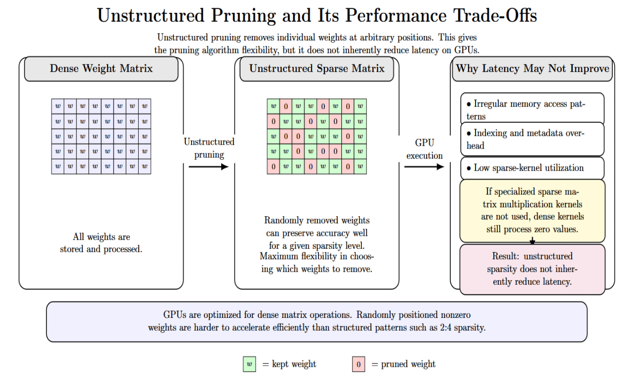
However, GPUs are designed to efficiently handle dense matrix operations. Sparse matrices with weights at random positions will result in irregular memory access patterns, indexing overhead, and low kernel utilization. If specialized sparse-matrix multiplication kernels are not used, dense matrix multiplication still processes zero values. As a result, unstructured sparsity does not inherently reduce latency.

Structured sparsity

Structured pruning eliminates weights in regular structures, such as rows, columns, blocks, channels, or fixed groups of weights. An example of a hardware-friendly structured pattern is 2:4 sparsity, also known as semi-structured sparsity. With 2: 4 sparsity, two values within a block of four contiguous weights are zero. This results in a 50% sparsity rate.

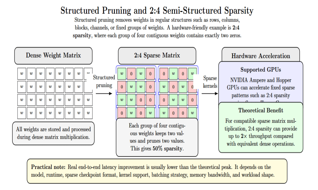
Supported GPUs can accelerate these fixed sparse patterns. NVIDIA’s Ampere GPU architecture added support for Sparse Tensor Cores for fine-grained structured sparsity, including the 2:4 pattern. In theory, they can provide up to 2× matrix multiplication throughput compared with equivalent dense operations. But in practice, end-to-end latency improvement varies based on model, runtime, kernels, and workload.

Traditional neural-network pruning workflows consisted of a three-step loop: Train a dense model. Remove less important weights. Fine-tune or retrain the sparse model to regain accuracy. Repeat until desired level of sparsity. Iterating this process can lead to very sparse networks, but it requires substantial computation.

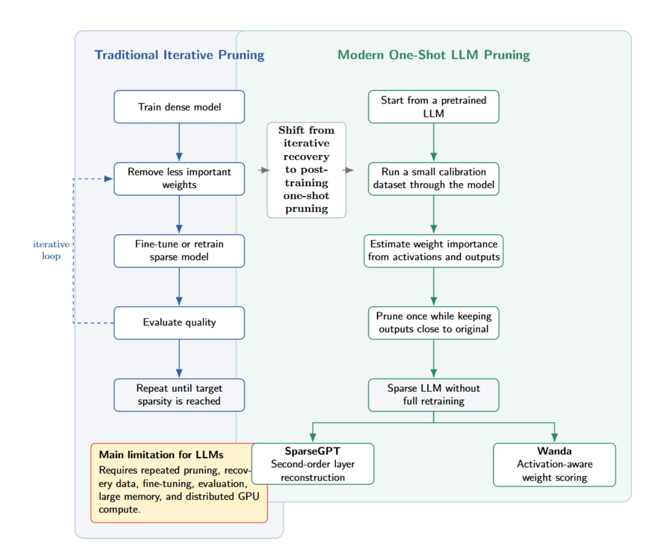
For billion-parameter LLMs, this pruning workflow is not easily done in practice. You’d have to load enormous models into memory and distributed GPU clusters, then prepare appropriate recovery data. After each pruning step, you would also need to run fine-tuning and evaluate model quality before moving to the next compression stage.

Another limitation of some older pruning methods is that they require expensive second-order approximations or iterative weight updates. These methods may still maintain accuracy, but are more challenging to scale to larger models as we shift from millions to billions of parameters.

Modern LLM pruning methods focus on post-training, one-shot pruning. Instead of iterative fine-tuning, they take a pretrained model and run a small calibration dataset through it to estimate which weights are less important. The model is then pruned so that its outputs are kept “close” to the original outputs on a representative set of inputs, without full retraining.

SparseGPT and Wanda are two notable methods of this category. SparseGPT estimates importance using second-order layer reconstruction; Wanda uses a simpler approach of activation-aware weight-importance scoring.

SparseGPT is a one-shot pruning method applicable to massive GPT-style models. It frames pruning as a layer-wise sparse regression problem. Given a linear layer with weights W and calibration activations X, we want to find a pruned matrix that minimizes reconstruction error:

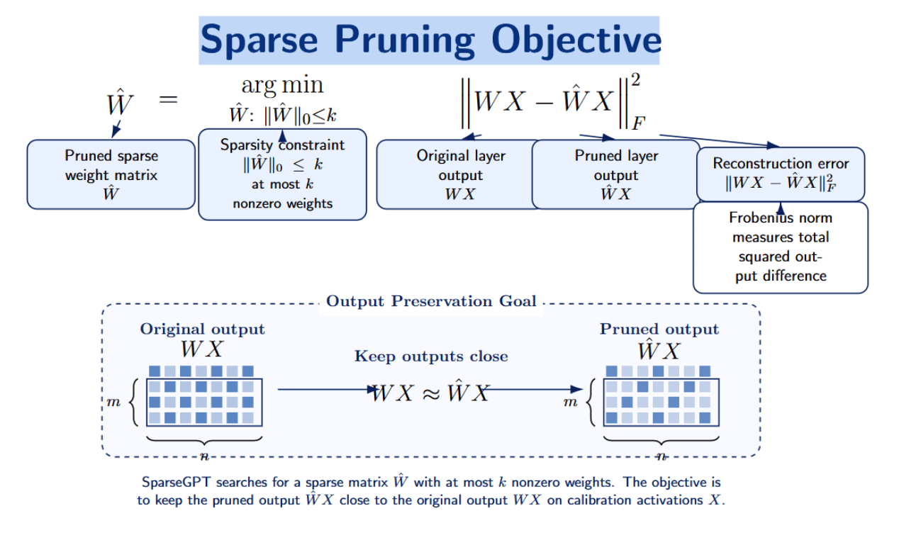
The outputs of the pruned layer should closely match those of the original layer for a given set of calibration data. SparseGPT tries to match this layer’s output rather than naively dropping the smallest weights. It uses second-order information calculated from calibration activations to approximate the impact of pruning on a layer’s output. After identifying which weights to prune, SparseGPT updates the remaining weights to compensate for the removed ones and minimize reconstruction error.

Why SparseGPT works well

SparseGPT balances accuracy and efficiency by combining several ideas:

• Second‑order sensitivity. Instead of simply pruning weights based on their magnitude, approximate Hessian information is used to rank weights by the impact their removal has on output reconstruction. This allows important weights that aren’t necessarily the largest to be kept.
• Layer‑wise processing. Remaining weights can be tweaked after pruning to reduce reconstruction error. This step allows model behavior to be maintained at higher levels of sparsity.
• Weight compensation. After pruning, the remaining weights can be adjusted to reduce reconstruction error. This step helps maintain model behavior at higher sparsity levels.
• Compatibility with patterns. SparseGPT supports unstructured pruning as well as semi‑structured pruning patterns like 2:4. In the case of 2:4, the algorithm considers each group of four weights and selects two to keep. This allows the pruning method to be applied to hardware that has specialized support for structured sparsity.

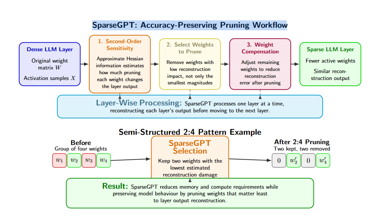
Thanks to these properties, SparseGPT maintains quality far better than naive methods when pruning aggressively. Its complexity is higher, but the authors show it scales to models with tens to hundreds of billions of parameters.

Wanda (Pruning by Weights and Activations) is an approach to lightweight pruning that was introduced as an alternative to reconstruction-based methods such as SparseGPT. Unlike these methods, it doesn’t involve solving a layer-wise reconstruction problem or estimating Hessians. Instead, it uses a simpler activation-aware importance score:

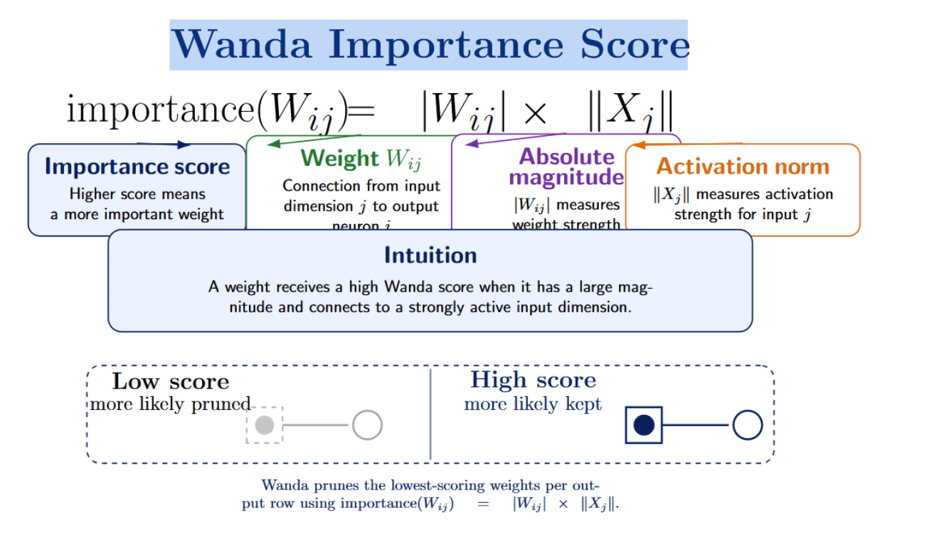
The intuition behind this score is that a weight will be important if it has a large magnitude and connects to an input dimension with strong activation. A weight with small magnitude or that connects to an input dimension with weak activation will be more likely to have a low importance score, and can therefore be pruned. Wanda ranks weights by removing those with the smallest activation-scaled magnitudes per-output basis. The authors highlight that Wanda requires zero retraining or weight updates - the pruned model can be used directly. Wanda heavily outperforms magnitude-based pruning and is competitive with more complex pruning methods in experiments run on LLaMA and LLaMA-2.

Why Wanda is attractive

Wanda’s simplicity yields several benefits:

• Ease of implementation. The algorithm requires only the collection of activation norms and the sorting of weights. There are no Hessian approximations or large regression problems to solve.
• Fast pruning pass. There is no weight update during pruning, so pruning massive models is orders of magnitude faster than SparseGPT. The Wanda authors claim Wanda is 5–10× faster than SparseGPT for 70B models trained on a single GPU(specifically H100).
• Competitive accuracy. Despite Wanda’s simplicity, it retains quality quite well for moderate levels of sparsity. On Llama‑2 models, unstructured pruning with Wanda achieves perplexity close to SparseGPT and is much better than pure magnitude pruning.
• Baseline for experimentation. Engineering teams should be able to run Wanda quickly to test how sparse models behave in their deployment stack before investing in more sophisticated techniques.

The trade‑off is that Wanda may lose accuracy faster than SparseGPT at very high sparsity ratios. It does not support weight compensation and is designed primarily for unstructured pruning, although the implementation includes options for 2:4 and 4:8 patterns.

Let’s consider the following table:

SparseGPT shines when you need to retain accuracy and have engineering resources available. Wanda is better for rapid experiments, lighter‑weight deployments, or when approximate answers are good enough. Many teams benchmark both approaches to find the sweet spot for their model, sparsity target, and hardware.

Deploying pruned LLMs involves both model‑level and infrastructure‑level considerations. A typical workflow looks like this:

1. Select the base model. Choose an open‑source model (e.g., Llama, Mistral, OPT, BLOOM) that suits your target application and has a compatible format you can work with (e.g., Hugging Face Transformers). Make sure the dense model fits in VRAM at least for calibration purposes.
2. Prepare the calibration dataset. SparseGPT and Wanda require only a small dataset that reflects the target workload. If you’re building a code assistant, use code prompts. If you’re building a support chatbot, use actual support conversations. Hundreds of samples are enough.
3. Choose sparsity level and pattern. You can start small at 20–30% to observe the effects. Moderate sparsity in the range of 40-50% provides significant memory savings with limited quality drops. For hardware acceleration, consider 2:4 or 4:8 patterns.
4. Apply the pruning method. SparseGPT method simply requires you to run the provided scripts against each model layer. The algorithm triggers the collection of activations, runs the sparse regression solver, and can optionally update weights. Wanda requires you to implement the importance metric against each linear projection. Each method only requires a single GPU. The runtime will scale with model size.
5. Save the sparse checkpoint. Simply store weights using the appropriate format. For unstructured sparsity, you can save weights and a mask. For 2: 4 sparsity, you’ll want to use compressed formats compatible with PyTorch or TensorRT. Record metadata such as model version, sparsity ratio, calibration data, pruning method, and data type.
6. Benchmark the pruned model. Measure perplexity and downstream task quality on relevant datasets or workloads. Evaluate VRAM usage, tokens per second, time‑to‑first token, inter‑token latency, and inference cost per million tokens. Measure both dense and sparse models under the same conditions.
7. Integrate into serving stack. When using structured sparsity, make sure the inference engine can load sparse weight formats and dispatch sparse kernels. Framework extensions like PyTorch’s to_ sparse_ semi_ structured can convert 2:4 masks and accelerate nn.Linear layers.
8. Monitor in production. Track latency, throughput, memory usage, and quality metrics. Adjust sparsity ratios or combine pruning with quantization and KV‑cache optimisations as needed.

Python example: implementing Wanda for a linear layer

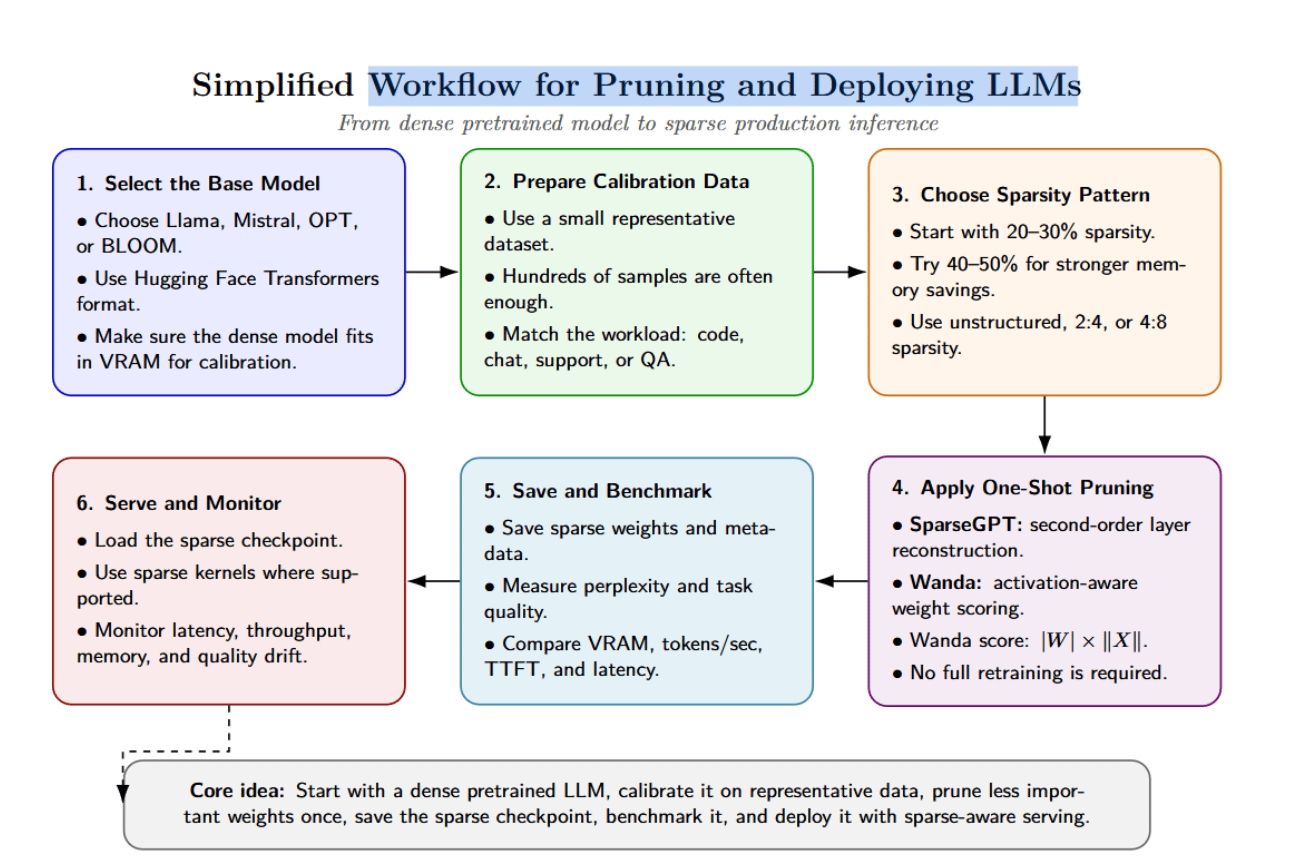
Below is a simplified PyTorch function that applies Wanda pruning to a single linear layer. In practice, you would extend this to all projection layers of the model and handle structured patterns.

import torch
import torch.nn as nn
@torch.no_grad()
def wanda_prune_linear(
    layer: nn.Linear,
    input_activations: torch.Tensor,
    sparsity: float = 0.5
):
    """
    Apply Wanda-style unstructured pruning to one Linear layer.


    Args:
        layer: PyTorch Linear layer.
        input_activations: Calibration activations with shape
            [batch, seq_len, hidden_dim] or [num_tokens, hidden_dim].
        sparsity: Fraction of weights to prune per output row.


    Returns:
        The pruned layer, modified in-place.
    """
    if not isinstance(layer, nn.Linear):
        raise TypeError("wanda_prune_linear expects an nn.Linear layer.")


    if not 0.0 <= sparsity <= 1.0:
        raise ValueError("sparsity must be between 0 and 1.")


    # Flatten activations to shape [n_tokens, input_dim]
    if input_activations.dim() == 3:
        X = input_activations.reshape(-1, input_activations.shape[-1])
    else:
        X = input_activations


    W = layer.weight


    if X.shape[-1] != W.shape[1]:
        raise ValueError(
            f"Activation dimension {X.shape[-1]} does not match "
            f"layer input dimension {W.shape[1]}."
        )


    # Compute L2 norm of each input dimension
    activation_norm = torch.norm(X, p=2, dim=0)


    # Compute Wanda importance scores: |W_ij| * ||X_j||
    scores = torch.abs(W) * activation_norm.unsqueeze(0)


    # Number of weights to prune per output row
    num_prune = int(W.shape[1] * sparsity)


    if num_prune == 0:
        return layer


    # Build pruning mask
    mask = torch.ones_like(W, dtype=torch.bool)


    for row in range(W.shape[0]):
        prune_indices = torch.topk(
            scores[row],
            k=num_prune,
            largest=False
        ).indices
        mask[row, prune_indices] = False


    # Apply mask in-place
    W.mul_(mask)


    return layer

# Example usage
device = "cuda" if torch.cuda.is_available() else "cpu"

hidden_dim = 4096
linear = nn.Linear(hidden_dim, hidden_dim, bias=False).half().to(device)

calibration_activations = torch.randn(
    4, 128, hidden_dim,
    device=device,
    dtype=torch.float16
)

pruned_layer = wanda_prune_linear(
    linear,
    calibration_activations,
    sparsity=0.5
)

zero_count = torch.sum(pruned_layer.weight == 0).item()
total_count = pruned_layer.weight.numel()

print(f"Sparsity: {zero_count / total_count:.2%}")

This is an example of simplified Wanda-style pruning for a single nn.Linear layer in PyTorch. Calibration activations are used to compute the L2 norm of every input dimension. Activation norms are multiplied by the absolute value of the weight to calculate Wanda importance scores. The lowest-scoring weights are pruned for each row of the output according to the desired sparsity ratio by multiplying by a binary mask in place. In this example, a half-precision linear layer is created. Random calibration activations are generated. The layer is pruned to 50% sparsity, and the final percentage of zeros in the weight is printed.

Evaluating pruned models requires metrics that capture both quality and efficiency:

• Perplexity and downstream accuracy show how pruning affects language modelling and task performance. SparseGPT authors report that GPT-family models can be pruned to >=50% sparsity in one shot without any retraining with minimal accuracy loss. They show that OPT-175B and BLOOM-176B both can reach 60% unstructured sparsity with a negligible increase in perplexity.
• VRAM usage reflects memory savings. If the inference stack stores pruned weights in compressed formats and uses sparse kernels, VRAM consumption drops roughly in proportion to sparsity.
• Throughput (tokens/second) and latency measure serving efficiency. Speedups require replacing dense kernels with sparse kernels; otherwise, zero weights still consume compute. For semi‑structured 2:4 sparsity, PyTorch’s tutorial demonstrates a 1.3× speedup for BERT on A100 GPU.
• Time‑to‑first token and inter‑token latency gauge user experience. A smaller memory footprint can reduce these latencies.
• Cost per million tokens connects engineering improvements to business value. Compression that halves memory and increases throughput can significantly lower cost per token.

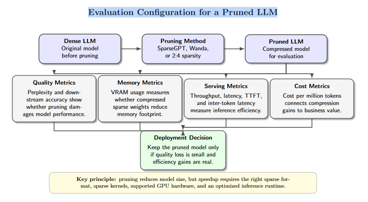
It is important to set realistic expectations: 50% sparsity does not guarantee 2× speedup. The real speedup depends on hardware support, kernel implementation, batch size, and whether the workload is dominated by weight computation or KV‑cache operations. Structured sparsity is easier to accelerate because hardware and software support specific patterns. Unstructured sparsity often requires custom CUDA kernels or frameworks like Triton.

Pruning is not just a model optimisation technique—it is an infrastructure problem. Several factors determine whether sparsity translates into speed:

• Checkpoint format. Storing zero weights in a dense tensor wastes storage and reduces potential memory savings. Semi-structured sparsity is stored in compressed formats, where non-zero elements are stored along with metadata describing their position. Libraries like cusparSELt provide kernels optimized for specific supported sparse formats.
• Kernel support. Dense matrix multiplication kernels do not skip zero weights. To gain speed, the runtime must dispatch sparse kernels that can exploit the sparse weight layout. PyTorch’s to_ sparse_semi_ structured method can transform weights that already have a supported semi-structured sparsity pattern into a sparse tensor datatype that unlocks sparse-kernel execution.
• NVIDIA Ampere and Hopper GPUs support sparse Tensor Cores, but only for hardware-friendly patterns such as 2:4 sparsity. Unstructured sparsity (i.e., random pruning) is harder to accelerate and may require general sparse GEMM libraries or writing custom kernels. Additionally, it often does not provide strong speedups unless the model is both extremely sparse and the runtime is optimized for sparsity.
• Batching and scheduling. Sparse matrix multiplication may be faster, but overall latency also depends on KV- cache management, batching, request scheduling, and memory bandwidth. In long-context or highly concurrent workloads, the KV cache can dominate memory usage, and reduce the practical benefit of weight pruning.
• Observability. It is essential to have good observability on latency, throughput, GPU utilization, memory usage, and quality. While sparsifying a model could reduce latency in a leaderboard benchmark, it might cause quality on user-facing tasks to fall below production standards.

The image below shows how pruning can speed up LLM inference only when the model, sparse checkpoint format, GPU kernels, and serving infrastructure are properly aligned. It uses a simple 2:4 sparsity example to show why pruning alone is not enough for real production gains.

Choose SparseGPT or Wanda when you want to reduce inference cost without retraining from scratch. Use them to fit larger models into smaller GPUs, to serve more models on a single GPU node, to reduce memory footprint and KV cache pressure. They can help to rapidly test compressed variants of your LLMs, prepare the models for edge deployment, and improve the economics of deploying open-source LLMs.

Don’t rely on pruning alone if your inference engine can’t exploit sparse weights, your workload accesses the KV cache most of the time, your model quality drops after pruning, or the deployment hardware doesn’t support sparse acceleration.

Choose SparseGPT if maintaining quality at a higher sparsity level is your primary goal. Choose Wanda if fast experimentation and low implementation complexity matter more.

The right production question is not simply: “Is the model sparse?” The better question is: “Does this sparse model reduce cost per useful token while preserving quality?”

• What is LLM pruning? LLM pruning is a compression technique that removes less important weights from a model. The goal is to reduce memory usage and inference cost while preserving model quality.

• What is the difference between SparseGPT and Wanda? SparseGPT uses second-order reconstruction to preserve layer outputs after pruning. Wanda uses a simpler activation-aware score based on weight magnitude and input activation norm, making it easier and faster to apply.

• Does pruning automatically make an LLM faster? No. Pruning only improves speed when the inference stack can exploit sparse weights through sparse formats, sparse kernels, and compatible hardware. If dense kernels still process zero weights, latency may not improve.

• When should I choose SparseGPT? Choosing SparseGPT when maintaining quality at higher sparsity levels is the main goal. It is more complex, but it is designed to preserve model behavior through reconstruction and weight compensation.

• When should I choose Wanda? Choose Wanda when fast experimentation, simplicity, and low implementation complexity matter more. It is a strong baseline for quickly testing how pruning affects a model before investing in more complex optimization.

SparseGPT and Wanda both illustrate that we can prune large language models after training without retraining. SparseGPT uses an involved reconstruction‑based metric with second‑order approximations to achieve this at scale while retaining accuracy. Wanda takes a much simpler activation‑aware approach, multiplying the weight by the input norm activation, enabling fast pruning with minimal engineering cost. Both projects result in sparse models that relieve memory pressure and (with the right kernels and hardware) improve inference throughput & lower latency.

Pruning isn’t the only consideration, though. Speedups and cost savings will only be realised with system‑level support for sparse formats, custom sparse kernels, smart memory optimisation and other techniques such as quantization and KV‑cache management. Inference stacks deployed in production will likely use a mix of strategies–pruning, quantization, caching, batching, speculative decoding, routing–to serve responsive AI services at the lowest possible cost. In that future, pruning will be a standard part of the LLM optimisation pipeline: not merely a research novelty but a practical tool for reducing cost per token and scaling AI services efficiently.

• SparseGPT: Massive Language Models Can Be Accurately Pruned in One-Shot
• A Simple and Effective Pruning Approach for Large Language Models
• Accelerating BERT with semi-structured (2:4) sparsity
• Estimating LLM Inference Memory Requirements
• Pruning LLMs by Weights and Activations