








You take a vision-language model to production and put it on the same GPU that’s been happily serving your text model: similar parameter count, the same serving stack, nothing different. The GPU shows 40% utilization, memory bandwidth is sitting at half capacity, and the tensor cores are barely warm. Yet the thing is slow: each request takes longer than it should, and the requests-per-second you can push through has fallen off compared to the text-only model you were running recently.
Nothing in the logs explains it.
No OOM errors, no runaway processes, no obvious resource fight. Just an expensive GPU quietly underperforming for no reason you can point to.
This is usually where teams start tuning, bump the batch size, change the sampling settings, and change the quantization config. Some of it helps a little, but none of it fixes the real problem, because the real problem isn’t in the config: it’s in the hardware contract you signed without reading.
A vision-language model doesn’t do one kind of work.
It does two, and those two kinds of work want opposite things from a GPU. Vision encoding is almost pure computation: millions of matrix multiplies, barely touching memory. Whereas, language decoding is the reverse: for every token it generates, it drags the model weights and a growing cache out of memory while the compute units are mostly idle. Putting both tasks on one GPU, which is what every standard deployment does, and you’ve committed to a permanent compromise: the encoder never gets the compute density it wants, the decoder never gets the memory bandwidth it wants, and you pay full freight for a GPU that’s underused in two different ways at once.
That’s the HBM tax or High Bandwidth Memory. And if you’re serving multimodal traffic at volume (high-resolution images, video, multi-image prompts), it’s eating a third or more of your inference budget. The good news is that the fix is well understood; it requires control over which GPU runs which phase, which is exactly the control most managed inference hides from you. We’ll get to how to do it on infrastructure you can actually rent (DigitalOcean GPU Droplets, specifically) toward the end. First, the mechanics.
A March 2026 paper by Donglin Yu (arXiv:2603.12707) is one of the first to put hard numbers to this, tracing where the inefficiency lives, why standard monitoring misses it, and what happens to cost and throughput when the two phases are finally pulled apart. It’s the backbone of what follows.
Vision-language models (VLMs) do two kinds of work with opposite hardware needs. Vision encoding is compute-heavy and barely touches memory. Language decoding is the reverse and it reads large amounts of memory for every token it generates. Putting both on one GPU permanently underserves both phases.
The HBM (High Bandwidth Memory) tax is the cost of that mismatch. Image tokens enter the KV (Key-Value) cache at the start of a request and stay there through every decode step. Every generated token pays a memory bandwidth cost for those image tokens, and that cost compounds under load.
Standard monitoring won’t show it. No single metric spikes. The GPU looks healthy. The tax shows up in the contention between resources, not the saturation of one.
The right fix is to cut at the modality boundary. Splitting after the vision encoder outputs its embedding before the language model starts transfers only ~4.5 MB per request (for LLaVA-7B) instead of the ~350 MB KV cache that stage-level disaggregation would require. That’s a 78× reduction, and the ratio gets better as models get deeper.
This works over ordinary cloud networking. A 4.5 MB embedding crosses a standard 25 Gbps private network in a few milliseconds, less than 1% of the encoding time. No NVLink or InfiniBand required.
The cost savings are real and measurable. The research validated ~40% savings from heterogeneous deployment (compute-dense GPU for encoding, HBM-rich GPU for decoding), with no latency regression.
The advantage grows over time. Deeper models and higher-resolution images both increase the gap between modality disaggregation and the alternatives. This isn’t a temporary workaround, it reflects a structural property of encoder-decoder architectures.
Before the numbers, it helps to picture what actually happens inside a vision-language model when a request comes in. There are two distinct jobs, in sequence:
The first is vision encoding. The model doesn’t see an image the way you do. It chops it into fixed-size patches (think of slicing a photo into a grid of tiles) and runs each tile through layers of math to turn it into a list of numbers the language side can work with. This is dense, back-to-back matrix multiplication, and the data it needs stays close to the processor. It barely reaches out to memory at all.
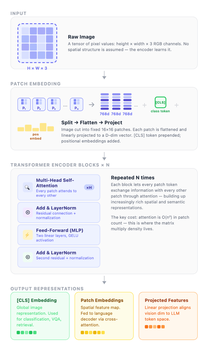
The second is language decoding. Once the image is encoded, the model generates its response one token at a time. For every token, it has to load its entire weight set plus everything generated so far (the KV cache) out of memory, do a small amount of math, emit one token, and repeat. It’s less like computing and more like reading a very long book one page at a time.
Two completely different kinds of work.
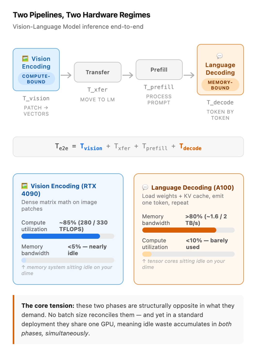
T_e2e = T_vision + T_xfer + T_prefill + T_decode
T_vision is encoding the image. T_xfer is moving the encoded output to the language model. T_prefill is processing the text prompt. T_decode is generating the response token by token, and in practice, that last phase is where most of the time and cost live.
What the measurements show: During vision encoding on an RTX 4090, the paper records over 85% utilization of the GPU’s compute (roughly 280 of 330 TFLOPS) while memory bandwidth sits below 5%. The GPU is pinned doing math; memory is nearly idle. Flip to language decoding on an A100 and the picture inverts: memory-bandwidth utilization crosses 80% (about 1.6 of 2 TB/s) while compute drops below 10%. Almost all the time goes to shuttling data in and out of memory, with barely any arithmetic.
These two phases are structurally opposite in what they demand. No batch size reconciles them. And yet in a standard deployment, they share one GPU, so during encoding, the memory system sits idle on your dime, and during decoding, the tensor cores sit idle on your dime. The waste is in both phases, at once, on the same card.
To understand the cost, look at the KV cache. That’s where vision tokens are stored, and they consume some of your most expensive resources.
Let us understand this better:
When a transformer processes a sequence, each attention layer computes three matrices for every token: Query (Q), Key (K), and Value (V). Attention works by having each token’s Q “look at” all previous tokens’ K/V pairs to decide what to attend to.
The expensive part: if you’re generating token by token, you’d recompute K and V for every previous token at every new step. That’s quadratic in cost as sequence length grows.
The KV cache is the fix - you compute K and V once per token and store them in memory. When generating the next token, you only compute K and V for that new token and append it to the cache. Previous tokens’ K/V matrices are just read from memory.
For each layer, for each token, you store two matrices (K and V). So the cache size scales with:
A rough formula for one sequence:
KV cache size = 2 × num_layers × seq_len × num_heads × head_dim × bytes_per_element
For Llama 3 70B (80 layers, 8 KV heads, head_dim 128, fp16): a single 128K-token sequence uses ~80GB - more than the model weights themselves.
Model weights are static - load once, reuse forever. The KV cache is dynamic and per-request. This is why:
With that foundation, “what the KV cache actually costs” becomes a story about VRAM pressure, throughput limits, and the tradeoffs operators make to serve long-context models at scale.
The cache exists because attention needs to look back. To generate token N, the model attends over the keys and values of every prior token, at every layer. Recomputing those each step would be quadratic, so you cache them. For a multi-head attention model, the size is:
D_KV = 2 · L · n_kv · d_h · s_ctx · b
Two tensors (keys and values), times layers L, times KV heads n_kv, times head dimension d_h, times context length s_ctx, times batch size b, times bytes per element.
Plug in a 7B MHA model (L=32, n_kv=32, d_h=128) at FP16, with a modest request: one 336×336 image through ViT-L/14 yields 576 vision tokens, plus 128 text tokens, for a context of 704. That’s roughly 350 MB of KV cache for a single request. Batch eight for prefill and you’re at about 2.8 GB before generating a single output token.
Now tie that to the image. Those 576 vision tokens aren’t a transient cost you pay during encoding and release. They’re written into the KV cache at prefill and they stay there for the entire decode loop. Every output token, attention sweeps back over all 576 of them. The image is conceptually “gone” (you’ve distilled it into embeddings), but its footprint in memory persists, and the bandwidth cost of re-reading it is paid on every step of generation.
This is where arithmetic intensity explains the damage. Arithmetic intensity is the ratio of compute performed to bytes moved. Decode has almost none: you move a huge amount of data to do a sliver of math, the definition of memory-bound. Stuffing the KV cache with hundreds of image tokens inflates the bytes-moved side of that ratio without adding any compute to justify it. You’re loading an already memory-starved phase with more memory traffic, for tokens that add context but no new arithmetic. The decode loop slows in direct proportion to how many image tokens you crammed in, and it pays that penalty once per generated token, every token. That’s the throughput collapse from the intro, expressed in bytes.
The natural reaction is: fine, disaggregate. Split the pipeline across devices so each phase runs where it’s happy. The paper surveys why the standard cuts fall short.
Stage-level disaggregation (EPD, Cauchy-style systems) - splits prefill from decode onto separate instances. Reasonable in spirit: prefill is compute-heavy, decode is memory-heavy. The catch is the cut point: after prefill, you have to migrate the entire KV cache to the decode instance, a transfer that scales as O(L · s_ctx), hundreds of megabytes to gigabytes per request. Moving that without wrecking latency demands NVLink or InfiniBand, which shuts consumer GPUs on ordinary networking out entirely. You haven’t removed the bottleneck; you’ve relocated it onto the interconnect and locked yourself into premium fabric.
Intra-node co-location (SpaceServe, UnifiedServe-style systems) - keeps everything on one GPU but multiplexes the two workloads spatially, so the idle resources of one phase get used by the other. It genuinely improves utilization, but it doesn’t change the cross-device communication structure, can’t pull in cheaper hardware for the compute-bound work, and doesn’t relieve the fundamental memory pressure at scale. You’re still serving decode out of one expensive memory budget.
Homogeneous serving (the vLLM baseline) is the workhorse - PagedAttention, continuous batching, careful memory management, all excellent, all worth using. But none of it addresses the hardware mismatch. Both phases still run on the same datacenter GPU, and you still pay for HBM bandwidth even when the active workload is encoder-heavy and bandwidth-agnostic.
The paper’s diagnosis of why these stop short is the sharp part: stage-level partitioning bakes in a language-only assumption. In a text-only LLM, the KV cache is the only meaningful intermediate state, so cutting around it is natural. Multimodal inference breaks that assumption. There’s now a second, very different intermediate (the vision embedding) with radically better transfer economics than the KV cache. The prior art was solving the right problem at the wrong boundary.
Here’s the load-bearing idea, and it’s clean once you see it.
The vision encoder’s output is a single embedding tensor of size O(N_v · d): visual token count times hidden dimension. That’s it. It does not grow with the language model’s depth L. The KV cache does, because every layer contributes its own keys and values. So if you partition at the modality boundary (between the vision encoder’s output and the language model’s input), the only thing that crosses the wire is that compact embedding. You never migrate a KV cache at all, because the cut happens before the cache exists.
The numbers aren’t subtle. For LLaVA-7B (576 vision tokens, d=4096) at FP16:
Embedding to transfer = 576 × 4096 × 2 bytes ≈ 4.5 MB
KV cache (the stage-level alternative) ≈ 350 MB
A 78x reduction in transferred bytes per request, purely from moving the cut point. The paper generalizes this (Theorem 1) as:
R = (2 · L · n_kv · d_h · s_ctx) / (N_v · d)
which under MHA collapses to a strikingly intuitive form:
R_MHA = 2L · (1 + s_text / N_v)
Two consequences fall out. The advantage scales with depth L: deeper models make stage-level disaggregation more expensive (a bigger cache to move) while the embedding stays the same size. And the ratio is independent of hidden dimension d: it cancels. So as models get deeper, modality-level disaggregation gets relatively more attractive, automatically.
Across architectures (the smaller figure reflects grouped-query attention, which shrinks n_kv and therefore the cache):
| Model | Transfer reduction (MHA / GQA) |
|---|---|
| LLaVA-7B | 78× |
| LLaVA-13B | 98× |
| LLaVA-34B | 147× / 21× |
| Qwen2.5-VL-7B | 64× / 12× |
| Qwen-VL-72B | 196× / 24× |
Even at the conservative GQA end, you’re moving an order of magnitude less data than a KV-cache migration would. The paper headlines the span as 12×–196× across current MLLMs: today’s GQA-heavy architectures cluster at the low end (12–24×), while MHA models and the deepest networks reach the top. The R_MHA figures for the GQA models are counterfactuals (what they would save under full multi-head attention), included to show how the advantage scales with depth.
You don’t need exotic interconnect**.** A 4.5 MB embedding over PCIe Gen4 x16 (~25 GB/s) clears in about 0.18 ms, against vision-encoding time the paper measures at ~6.8 s for a batch of 128 images. The reported ratio is T_xfer / T_vision < 0.003 across every architecture tested: the transfer is a rounding error against the work itself. No NVLink, no InfiniBand. And as we’ll see, the embedding is small enough that it survives not just PCIe but an ordinary cloud private network, which is what opens this up on real infrastructure.
The reason to care is the invoice.
The paper lays out a hardware asymmetry that practitioners feel but rarely price out. An RTX 4090 (~$3k, ~330 TFLOPS FP16) roughly matches an A100 (~$16k, ~312 TFLOPS) on raw compute, about 3.3× better FLOPs per dollar. Where the A100 pulls ahead is memory: ~2 TB/s of HBM versus the 4090’s ~1 TB/s, and far more of it. So the two cards aren’t “better” and “worse.” They’re specialists. One is a compute bargain that’s memory-poor; the other is a memory powerhouse you overpay for if all you need is FLOPs.
Map that onto the two phases and the assignment writes itself. Compute-bound, bandwidth-agnostic vision encoding belongs on the cheaper compute-dense card. Memory-bandwidth-bound, HBM-critical language decoding belongs on the datacenter card. Stop running the encoder on hardware you’re renting for its bandwidth, and stop running decode on hardware that can’t feed it.
The paper builds a closed-form cost model around this and validates it: it predicted 31.4% savings from heterogeneous deployment and measured 40.6%. As a budget decision, a ~$38k heterogeneous cluster delivered better Tokens-per-dollar than a ~$64k homogeneous one: roughly 37% better economics on identical workloads, with no latency regression. That’s not a single-digit tuning win. It’s a different cost structure, available because each phase finally runs on the silicon it wants.
Two honest caveats before you wire this up. First, those exact dollar figures are the paper’s RTX 4090 / A100 pairing. The structure of the savings (cheap compute card for encode, HBM card for decode) is what transfers, the precise percentage will depend on your model, your traffic mix, and the specific cards you choose. Second, the gain is real only when your workload is genuinely phase-separable at volume, which is the audience question we’ll come back to.
To prove the theory outside a spreadsheet, the paper builds a serving system, HeteroServe, around four ideas worth understanding even if you never run that exact stack.
Modality-level partitioning- Compute-dense GPUs run the vision encoder; HBM-heavy GPUs run the language model. Only embeddings cross the link between them: the cut from the previous section, made operational.
An embedding-only transfer protocol- Real models don’t emit a fixed token count: Qwen2.5-VL, for instance, produces a variable N_v depending on image resolution, up to ~2048 tokens. The system uses dynamic buffer allocation to absorb that. The economics still hold at the top of the range: 2048 tokens is ~14 MB, still roughly 6× smaller than the corresponding KV cache. “Transfer is negligible” is robust, not a best-case artifact.
Cross-type work stealing- The elegant bit for messy real traffic. A pure modality split has an obvious failure mode: what do your encoder GPUs do when a burst of text-only requests arrives and there’s nothing to encode? They’d sit idle. So when encoder GPUs have no vision work, they steal decode work from the language pool, recovering utilization that would otherwise evaporate, without the role-switching complexity that makes prefill/decode-swapping systems brittle.
Engine optimizations, kept separate on purpose- CUDA Graph-accelerated decoding, packed prefill, lazy KV allocation: the usual high-leverage tricks. The paper deliberately isolates these from the architectural contribution so the two don’t get conflated: on identical 4×A100 hardware, these optimizations alone lift throughput up to 54% over a vLLM v0.3.0 baseline. That’s a separate axis from the heterogeneity story. The cost win from modality disaggregation stacks on top of good engine hygiene; it doesn’t depend on it.
Everything above is hardware-agnostic theory. Here’s how it lands on infrastructure you can actually rent, and where the paper’s same-box assumption has to be adapted.
The paper’s elegant beat is “two cards, one PCIe link, in one box.” On a public cloud you generally don’t compose a heterogeneous multi-card box yourself; DigitalOcean GPU Droplets are single-GPU-class virtual machines you spin up independently. So the practical realization isn’t same-box PCIe: it’s two Droplets on the same private network, one tier for encode and one for decode, with embeddings crossing the wire between them. The good news is that the embedding is small enough that this works.
The hardware tiers map cleanly**.** DigitalOcean’s compute-dense, cost-efficient cards are the Ada-generation parts: NVIDIA L40S and RTX 6000 Ada (48 GB each), and RTX 4000 Ada (20 GB). These are the natural home for the compute-bound vision encoder, DigitalOcean positions the L40S at up to ~1.7× an A100 for AI workloads, and its modest memory is a non-issue here because encoding barely touches bandwidth. The HBM-heavy decode tier is the datacenter lineup: H100 (80 GB), H200 (141 GB, marketed at up to 2× H100 inference on memory-bound work), and the AMD Instinct MI300X / MI325X / MI350X parts with very large, high-bandwidth memory. In other words: L40S or RTX 6000 Ada for the encoder pool, H100 or H200 for the decoder pool. DigitalOcean’s own vLLM GPU-sizing guide reaches the same split from the workload side: high-bandwidth cards for memory-bound decode, high-compute cards for everything else.
Does the transfer survive a network hop instead of PCIe? This is the load-bearing question, so let’s do the arithmetic. Every GPU Droplet comes with 25 Gbps private networking, roughly 3 GB/s, call it ~2–2.5 GB/s sustained after real-world overhead. That’s about 8× slower per byte than the paper’s in-box PCIe. But the embedding is tiny:
So the paper’s sub-0.3% PCIe figure becomes low-single-digit-percent over DigitalOcean’s private network. The whole reason the modality boundary is the right cut is that it makes the transfer small enough to tolerate ordinary networking, which is exactly why this is feasible on a cloud where you don’t get NVLink between separate instances. (One practical constraint: keep both Droplet pools in the same datacenter region so they share that private network; GPU Droplets are available in several regions including NYC, Toronto, and Atlanta. One AMD-specific wrinkle worth planning around: the Instinct MI350X launched in Atlanta (ATL1) only, so if you want an AMD decoder pool today, both the encoder and decoder pools need to live in ATL1 to keep that private link.)
The reason you can build this on GPU Droplets at all is that they give you GPU-level control: you choose the card per pool, you place the instances, you own the orchestration between them. You can wire the two pools together over the private VPC network, front them with your own scheduler, and manage the whole thing through the API, Terraform, or Kubernetes. If you’d rather not hand-tune the decode tier, DigitalOcean’s Inference Optimized Image ships a pre-tuned vLLM stack (speculative decoding, FP8, FlashAttention-3, paged attention) across the H100, L40S, and RTX 6000 Ada tiers, and reports up to a 143% throughput gain over an untuned baseline: that’s the “good engine hygiene” layer the paper keeps separate, available out of the box on the same cards you’d use for the decode pool. For teams that want dedicated capacity rather than per-second instances, Bare Metal GPUs give you the whole machine.
This whole argument cuts against fully managed, serverless inference, and that deserves an honest assessment rather than a dismissal. The reason serverless can’t capture this saving is structural: the entire value proposition of serverless is that you don’t think about the hardware. You can’t ask a serverless endpoint to run your encoder on a compute-dense card and your decoder on a bandwidth-dense one, because making those placement decisions for you is the point of the product.
For a large fraction of teams, that’s the right trade. If you’re prototyping, if your multimodal volume is light, or if you don’t want to own a scheduler and two GPU pools, the operational simplicity of a serverless endpoint from DigitalOcean is worth far more than a cost optimization you’d spend engineering time chasing. The modality-split architecture earns its keep when three things are true at once: you serve multimodal traffic at enough volume that a ~30–40% inference-cost delta is real money; your workloads are image- or video-heavy, so KV-cache inflation bites hard; and you have the appetite to own your serving topology rather than rent it as a black box. Below that bar, stay serverless. Above it, the control that GPU Droplets give you is the thing that unlocks the saving, and the two products aren’t really competitors so much as the right answers to different scales.
You don’t have to take any of this on faith. The HBM tax is directly observable, and quantifying it in your own deployment is the right first move before you change any infrastructure.
Run the isolation experiment**.** Hold the LLM backbone fixed and vary only the visual input: (a) text only, (b) one low-resolution image, © one high-resolution image, (d) multiple images. Plot inter-token latency against image-token count. The slope of that line is the tax: the per-image-token cost your decode loop pays on every step.
What to instrument:
Tools that already give you most of this: vLLM’s Prometheus metrics expose KV-cache utilization and request-queue depth; NVIDIA Nsight Compute gives per-kernel bandwidth so you can attribute traffic to phases; a custom harness with controlled batch sizes closes the gap. DigitalOcean’s vLLM sizing guide walks through reading TTFT, ITL, and KV-cache pressure if you want a checklist.
What the data should reveal: under concurrent load, throughput degrades faster than linearly with image-token count. That’s the signature. It’s super-linear because HBM bandwidth is shared and contended, and the decode loop pays the inflated KV-cache cost on every token for every request in the batch at once. Linear would mean each image costs a fixed amount; super-linear means the images are fighting each other for bandwidth: the tax, observed in the wild.
The reason this matters past LLaVA and Qwen-VL is that the core advantage is a property of the architecture, not of vision specifically.
The asymmetry is simple: an encoder produces output that’s O(1) per layer (a fixed embedding, regardless of decoder depth) while a decoder accumulates O(L) of KV state. Any pairing with that shape benefits from the same analysis. Audio encoders like Whisper feeding a language model: same structure, same cut. Video encoders, which produce enormous token counts and would make a KV-cache migration brutal: same cut, bigger payoff. Multimodal models with several encoder branches: each branch is another O(1)-per-layer output you can partition off cheaply.
And the trend lines compound the advantage over time. Models keep getting deeper, which raises L and grows the transfer ratio in modality-disaggregation’s favor. Compute density on cheaper cards keeps climbing faster than interconnect bandwidth, widening the gap between cheap FLOPs and expensive bytes. The paper isn’t describing a quirk of one model generation: it’s describing a structural property of encoder-decoder multimodal systems that gets more true as both hardware and models advance.
Come back to the anomaly we opened with: the model that crawled while every dashboard insisted the GPU was fine. You can explain it precisely now. Image tokens enter the KV cache at prefill and stay there through every decode step. HBM bandwidth, the single scarcest resource in language decoding, gets split between the model weights and an ever-growing cache now carrying hundreds of image tokens that contribute memory traffic but no arithmetic. The GPU looked healthy because no single counter was pegged. The tax is paid in the contention between resources, not the saturation of any one of them.
The fix is a question about where in the inference graph you draw the line. The research says the modality boundary (the seam between vision encoder and language model) is the provably optimal place to draw it. Cut there and you reduce cross-device transfer by 12× to 196× depending on architecture and attention scheme (the GQA-heavy models that dominate today’s deployments at the lower end, deeper and MHA models at the upper), you make ordinary networking sufficient for the transfer, and you open up a cost structure (on the order of 30–40% cheaper in the source research) that homogeneous deployments structurally cannot reach. On DigitalOcean, that means an Ada-class encoder pool, an HBM-class decoder pool, and 25 Gbps of private network between them.
The GPU was never the problem. Asking one GPU to be two different machines was.
What is the HBM tax?
HBM stands for High Bandwidth Memory the fast memory on a GPU. The “HBM tax” refers to the hidden performance and cost penalty you pay when a vision-language model runs both image encoding and text generation on the same GPU. The two phases need different things from the hardware, so neither gets what it needs.
My GPU metrics look normal. How do I know if I’m paying this tax?
Run the same model with different inputs text only, one small image, one large image, multiple images and measure how long each generated token takes as image size goes up. If the per-token latency grows faster than linearly with image token count, you’re paying the tax
What is a KV cache and why does it matter here?
KV stands for Key-Value. When a language model generates text, it stores intermediate results for every token it has already processed so it doesn’t have to recompute them. This stored data is the KV cache. Image tokens get added to this cache and stay there for the entire generation so every output token has to read all of them from memory, again and again.
Why can’t I fix this by tuning batch size or quantization?
Those settings help at the margins, but they don’t address the root cause. The problem is that vision encoding and language decoding want fundamentally different hardware. No config change reconciles that on a single GPU.
What does modality-level disaggregation mean?
It means running the vision encoder on one GPU and the language model on a separate GPU. The only thing transferred between them is the encoder’s output, embedding a small, fixed-size tensor rather than the full KV cache. This makes the transfer fast enough to work over a standard cloud private network.
Do I need special hardware or interconnects like NVLink?
No. The embedding transferred between GPUs is small enough (a few megabytes) that a standard 25 Gbps private network handles it with negligible overhead. This is what makes the approach practical on standard cloud infrastructure.
When does this actually make sense to implement?
When three things are true: you’re serving enough multimodal traffic that a 30–40% cost reduction is meaningful, your requests are image- or video-heavy (not occasional), and you’re willing to manage your own serving setup. If you’re early-stage or low-volume, a managed serverless endpoint is simpler and likely the better trade-off.
Does this apply to models beyond vision-language models?
Yes. Any architecture where a fixed-output encoder feeds a depth-scaling decoder has the same structure. Audio models, video models, and multi-encoder multimodal systems all benefit from the same analysis.
 This work is licensed under a Creative Commons Attribution-NonCommercial- ShareAlike 4.0 International License.
此内容由惯性聚合(RSS阅读器)自动聚合整理,仅供阅读参考。 原文来自 — 版权归原作者所有。