








With massive data volumes growing at exponential rates, we need to find scalable methods to process them and find insights. The world of data entered the Zettabyte era several years ago. What’s a Zettabyte? Well, it is enough storage for 30 billion 4K movies, or 60 billion video games, or 7.5 trillion MP3 songs.
Today, the total amount of data created, captured, copied, and consumed globally is in the order of 100 Zettabytes and just keeps growing.
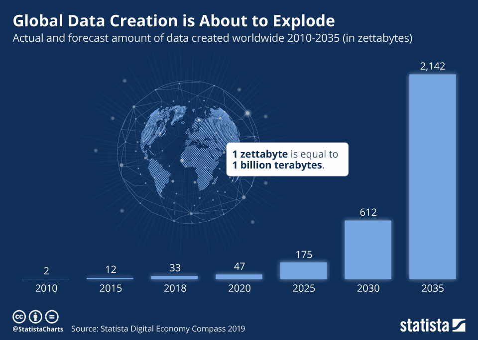
Through 2035, global data creation is projected to grow to more than 2,142 Zettabytes. From 2020, the growth was higher than previously expected caused by increased demand due to the COVID-19 pandemic, as more people worked and learned from home and used more home entertainment options.
Although this might seem overwhelming, the good news is that we can turn to machines for help: There are many different Machine Learning algorithms to discover patterns in big data that lead to actionable insights.
Depending on the way the algorithm “learns” about data to make predictions, we classify them into two groups, each proving one different type of learning:
Under unsupervised learning, all the objects in the same group (cluster) should be more similar to each other than to those in other clusters; data points from different clusters should be as different as possible. Clustering allows you to find and organize data into groups that have been formed organically, rather than defining groups before looking at the data.
While this article will focus most closely on K-means, there are other powerful types of clustering that can be used as well. Let’s take a look at the main ones like hierarchical, density-based, and partitional clustering.
Cluster assignments are determined by building a hierarchy. This is implemented by either a bottom-up or a top-down approach:
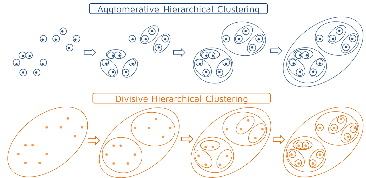
The agglomerative case starts with every object being a cluster and, in the next steps, merges them with the two closest clusters. The process finishes with every object in one cluster. The divisive algorithm, contrastingly, starts with every object in one cluster and ends with every object in individual clusters.
These methods produce a tree-based hierarchy of points called a dendrogram. The number of clusters “k” is often predetermined by the user, and clusters are assigned by cutting the dendrogram at a specified depth that results in “k” groups of smaller dendrograms.
Hierarchical Clustering returns an output (typically as a dendrogram like the right figure) from which the user can decide the appropriate number of clusters (either manually or algorithmically). If done manually, the user may cut the dendrogram where the merged clusters are too far apart (represented by long lines in the dendrogram). Alternatively, the user can just return a specific number of clusters.
Unlike other clustering techniques, hierarchical clustering is a deterministic process, which means that assignments won’t change when you run an algorithm multiple times on the same input data. Hierarchical clustering methods often reveal the finer details about the relationships between data objects and provide interpretable dendrograms. On the other hand, they’re computationally expensive with respect to algorithm complexity and sensitive to noise and outliers.
Under this category, cluster assignments are determined based on the density of data points in a region and assigned where there are high densities of data points separated by low-density regions.
Unlike other clustering categories, this approach doesn’t require the user to specify the number of clusters. Instead, there is a distance-based parameter that acts as a tunable threshold and determines how close points must be to be considered a cluster member.
Density-Based Clustering algorithms like DBSCAN don’t require a preset number of clusters. It also identifies outliers as noises unlike others that simply throws them into a cluster even if the data point is very different. Additionally, it is able to find arbitrarily sized and arbitrarily shaped clusters quite well.
Density-based clustering methods excel at identifying clusters of nonspherical shapes, and they are resistant to outliers. Nevertheless, they aren’t well suited for clustering in high-dimensional spaces (since density of data points is very low in those spaces), and they are not able to produce clusters of differing density.
With this method, data objects are divided into non-overlapping groups: No object can be a member of more than one cluster, and every cluster must have at least one object.
Like in hierarchical clustering, the user needs to define the number of clusters “k”, which ultimately produces non-deterministic results: Partitional clustering produces different results from two or more separate runs even if the runs were based on the same input.
This clustering method works very well when clusters have a spherical shape (due to its fixed distance norm), and they’re scalable with respect to algorithm complexity. However, they’re not well suited for clusters with complex shapes and different sizes, and they break down when used with clusters of different densities, since it doesn’t employ density parameters.
Partitional clustering algorithms deal with the data space and focus on creating a certain number of divisions of the space.
K-means is an example of a partitional clustering algorithm. Once the algorithm has been run and the groups are defined, any new data can be easily assigned to the existing groups. K-means is an extremely popular clustering algorithm, widely used in tasks like behavioral segmentation, inventory categorization, sorting sensor measurements, and detecting bots or anomalies.
From the universe of unsupervised learning algorithms, K-means is probably the most recognized one. This algorithm has a clear objective: partition the data space in such a way so that data points within the same cluster are as similar as possible (intra-class similarity), while data points from different clusters are as dissimilar as possible (inter-class similarity).
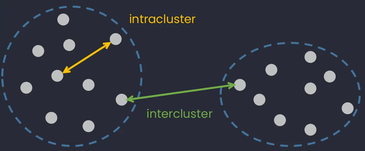
An illustration of inter-cluster and intra-cluster distance.
In K-means, each cluster is represented by its center (called a “centroid”), which corresponds to the arithmetic mean of data points assigned to the cluster. A centroid is a data point that represents the center of the cluster (the mean), and it might not necessarily be a member of the dataset. This way, the algorithm works through an iterative process until each data point is closer to its own cluster’s centroid than to other clusters’ centroids, minimizing intra-cluster distance at each step. But how?
K-means searches for a predetermined number of clusters within an unlabelled dataset by using an iterative method to produce a final clustering based on the number of clusters defined by the user (represented by the variable K). For example, by setting “k” equal to 2, your dataset will be grouped in 2 clusters, while if you set “k” equal to 4 you will group the data in 4 clusters.
K-means triggers its process with arbitrarily chosen data points as proposed centroids of the groups and iteratively recalculates new centroids in order to converge to a final clustering of the data points. Specifically, the process works as follows:
The figure shows the centroids updating through the first five iterations from two different runs of the K-means algorithm on the same dataset. The purpose of this figure is to show that the initialization of the centroids is an important step.
How do you choose the right value of “k”? When you define “k” you are telling the algorithm how many centroids you want, but how do you know how many clusters to produce?
One popular approach is testing different numbers of clusters and measuring the resulting Sum of Squared Errors (SSE), choosing the “k” value at which an increase will cause a very small decrease in the error sum, while a decrease will sharply increase the error sum. This point that defines the optimal number of clusters is known as the “elbow point”.
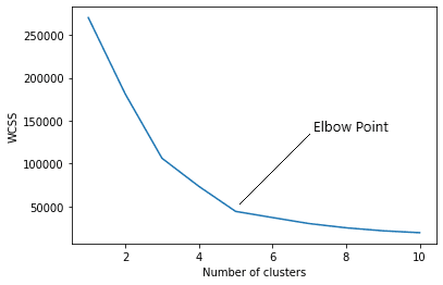
As the number of clusters increases, the Sum of Squared Errors within clusters will start to decrease. The error value is largest when “k” = 1. We can see that the graph will rapidly change at a point,thus creating an elbow shape. From this point, the graph starts to move almost parallel to the X-axis. The “k” value corresponding to this point is the optimal number of clusters.
Another alternative is to use the Silhouette Coefficient metric. This coefficient is a measure of cluster cohesion and separation, frequently used in unsupervised learning problems. It quantifies how well a data point fits into its assigned cluster based on two factors:
Silhouette coefficient values range between -1 and 1, meaning that well-defined clusters result in positive values of this coefficient, while incorrect clusters will result in negative values.
We can use a Silhouette plot to display a measure of how close each point in one cluster is to a point in the neighboring clusters and thus provide a way to assess parameters like the number of clusters visually.
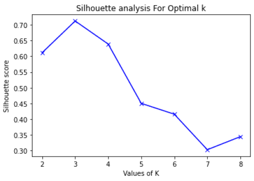
Using the above Silhouette analysis, we can choose an optimal k value as 3 because the average silhouette score is higher and indicates that the data points are optimally positioned.
K-means presents huge advantages, since it scales to large data sets, is relatively simple to implement, guarantees convergence, can warm-start the positions of centroids, it easily adapts to new examples, and generalizes to clusters of different shapes and sizes, such as elliptical clusters.
But as any other Machine Learning method, it also presents downsides. The most obvious one is that you need to define the number of clusters manually, and, although we showed some ways to find the optimal “k”, this is a decision that will deeply affect the results.
Also, K-means is highly dependent on initial values. For low values of “k”, you can mitigate this dependence by running K-means several times with different initial values and picking the best result. As “k” increases, you need advanced versions of K-means to pick better values of the initial centroids (called K-means seeding). K-means produces clusters with uniform sizes (in terms of density and quantity of observations), even though the underlying data might behave in a very different way. Finally, K-means is very sensitive to outliers, since centroids can be dragged in the presence of noisy data.
K-means is highly flexible and can be used to cluster data in lots of different domains. It also can be modified to adapt it to specific challenges, making it extremely powerful. Whether you’re dealing with structured data, embeddings, or any other data type, you should definitely consider using K-means.
此内容由惯性聚合(RSS阅读器)自动聚合整理,仅供阅读参考。 原文来自 — 版权归原作者所有。