


Facebook AI Similarity Search (Faiss) is one of the most popular implementations of efficient similarity search, but what is it — and how can we use it?
What is it that makes Faiss special? How do we make the best use of this incredible tool?
Note: Pinecone lets you implement vector search into your applications with just a few API calls, without knowing anything about Faiss. However, you like seeing how things work, so enjoy the guide!
Start using Pinecone for free
Pinecone is the developer-favorite vector database that's fast and easy to use at any scale.
Fortunately, it’s a brilliantly simple process to get started with. And in this article, we’ll explore some of the options FAISS provides, how they work, and — most importantly — how Faiss can make our search faster.
Check out the video walkthrough here:
Key Terms Glossary
Before diving in, here's a quick reference for the key acronyms and concepts used throughout this article:
| Term | Full Name | Description |
|---|---|---|
| Faiss | Facebook AI Similarity Search | An open-source library developed by Meta (Facebook) AI Research for efficient similarity search and clustering of dense vectors. |
| IVF | Inverted File Index | An indexing technique that partitions the vector space into Voronoi cells (clusters). At query time, only the nearest cell(s) are searched rather than the full index, dramatically speeding up approximate nearest-neighbor retrieval. |
| PQ | Product Quantization | A vector compression technique that splits each vector into sub-vectors, clusters each sub-vector set independently, and replaces each sub-vector with a centroid ID. This reduces memory usage and speeds up distance calculations at the cost of some accuracy. |
| IVFFlat | Inverted File Index (Flat) | Combines IVF partitioning with exact (flat) distance calculations within each cell. Faster than a pure flat index while maintaining good accuracy. |
| IVFPQ | Inverted File Index with Product Quantization | Combines IVF partitioning with PQ-compressed vectors. The most memory-efficient and fastest option, with a modest accuracy trade-off. |
| L2 | L2 (Euclidean) Distance | A distance metric measuring the straight-line distance between two vectors in space. Smaller L2 distance = more similar vectors. |
| nlist | Number of Voronoi Cells | A parameter that controls how many partitions the IVF index is divided into. More cells = finer partitioning and faster search, but requires more training data. |
| nprobe | Number of Cells to Search | A parameter that controls how many neighboring Voronoi cells are searched at query time. Higher values improve recall at the cost of speed. |
What is Faiss?
Before we get started with any code, many of you will be asking — what is Faiss?
Faiss is a library — developed by Facebook AI — that enables efficient similarity search.
So, given a set of vectors, we can index them using Faiss — then using another vector (the query vector), we search for the most similar vectors within the index.
Now, Faiss not only allows us to build an index and search — but it also speeds up search times to ludicrous performance levels — something we will explore throughout this article.
Building Some Vectors
The first thing we need is data, we’ll be concatenating several datasets from this semantic test similarity hub repo. We will download each dataset, and extract the relevant text columns into a single list.
In[1]:
import requests
from io import StringIO
import pandas as pd
The first dataset is in a slightly different format:In[4]:
res = requests.get('https://raw.githubusercontent.com/brmson/dataset-sts/master/data/sts/sick2014/SICK_train.txt')
# create dataframe
data = pd.read_csv(StringIO(res.text), sep='\t')
data.head()
Out[4]:
   pair_ID                                         sentence_A  \
0        1  A group of kids is playing in a yard and an ol...
1        2  A group of children is playing in the house an...
2        3  The young boys are playing outdoors and the ma...
3        5  The kids are playing outdoors near a man with ...
4        9  The young boys are playing outdoors and the ma...

                                          sentence_B  relatedness_score  \
0  A group of boys in a yard is playing and a man...                4.5
1  A group of kids is playing in a yard and an ol...                3.2
2  The kids are playing outdoors near a man with ...                4.7
3  A group of kids is playing in a yard and an ol...                3.4
4  A group of kids is playing in a yard and an ol...                3.7

  entailment_judgment
0             NEUTRAL
1             NEUTRAL
2          ENTAILMENT
3             NEUTRAL
4             NEUTRAL
In[5]:
# we take all samples from both sentence A and B
sentences = data['sentence_A'].tolist()
sentences[:5]
Out[5]:
['A group of kids is playing in a yard and an old man is standing in the background',
 'A group of children is playing in the house and there is no man standing in the background',
 'The young boys are playing outdoors and the man is smiling nearby',
 'The kids are playing outdoors near a man with a smile',
 'The young boys are playing outdoors and the man is smiling nearby']
In[6]:
# we take all samples from both sentence A and B
sentences = data['sentence_A'].tolist()
sentence_b = data['sentence_B'].tolist()
sentences.extend(sentence_b)  # merge them
len(set(sentences))  # together we have ~4.5K unique sentences
This isn't a particularly large number, so let's pull in a few more similar datasets.In[7]:
urls = [
    'https://raw.githubusercontent.com/brmson/dataset-sts/master/data/sts/semeval-sts/2012/MSRpar.train.tsv',
    'https://raw.githubusercontent.com/brmson/dataset-sts/master/data/sts/semeval-sts/2012/MSRpar.test.tsv',
    'https://raw.githubusercontent.com/brmson/dataset-sts/master/data/sts/semeval-sts/2012/OnWN.test.tsv',
    'https://raw.githubusercontent.com/brmson/dataset-sts/master/data/sts/semeval-sts/2013/OnWN.test.tsv',
    'https://raw.githubusercontent.com/brmson/dataset-sts/master/data/sts/semeval-sts/2014/OnWN.test.tsv',
    'https://raw.githubusercontent.com/brmson/dataset-sts/master/data/sts/semeval-sts/2014/images.test.tsv',
    'https://raw.githubusercontent.com/brmson/dataset-sts/master/data/sts/semeval-sts/2015/images.test.tsv'
]
In[8]:
# each of these dataset have the same structure, so we loop through each creating our sentences data
for url in urls:
    res = requests.get(url)
    # extract to dataframe
    data = pd.read_csv(StringIO(res.text), sep='\t', header=None, error_bad_lines=False)
    # add to columns 1 and 2 to sentences list
    sentences.extend(data[1].tolist())
    sentences.extend(data[2].tolist())
Out[8]:
b'Skipping line 191: expected 3 fields, saw 4\nSkipping line 206: expected 3 fields, saw 4\nSkipping line 295: expected 3 fields, saw 4\nSkipping line 695: expected 3 fields, saw 4\nSkipping line 699: expected 3 fields, saw 4\n'
b'Skipping line 104: expected 3 fields, saw 4\nSkipping line 181: expected 3 fields, saw 4\nSkipping line 317: expected 3 fields, saw 4\nSkipping line 412: expected 3 fields, saw 5\nSkipping line 508: expected 3 fields, saw 4\n'
Next, we remove any duplicates, leaving us with 14.5K unique sentences. Finally, we build our dense vector representations of each sentence using the sentence-BERT library.
In[6]:
# remove duplicates and NaN
sentences = [word for word in list(set(sentences)) if type(word) is str]
In[7]:
from sentence_transformers import SentenceTransformer
# initialize sentence transformer model
model = SentenceTransformer('bert-base-nli-mean-tokens')
# create sentence embeddings
sentence_embeddings = model.encode(sentences)
sentence_embeddings.shape
Now, building these sentence embeddings can take some time — so feel free to download them directly from here (you can use this script to load them into Python).
Plain and Simple
We’ll start simple. First, we need to set up Faiss. Now, if you’re on Linux — you’re in luck — Faiss comes with built-in GPU optimization for any CUDA-enabled Linux machine.
MacOS or Windows? Well, we’re less lucky.
(Don’t worry, it’s still ludicrously fast)
So, CUDA-enabled Linux users, type conda install -c pytorch faiss-gpu. Everyone else, conda install -c pytorch faiss-cpu. If you don’t want to use conda there are alternative installation instructions here.
Once we have Faiss installed we can open Python and build our first, plain and simple index with IndexFlatL2.
IndexFlatL2
IndexFlatL2 measures the L2 (or Euclidean) distance between all given points between our query vector, and the vectors loaded into the index. It’s simple, very accurate, but not too fast.
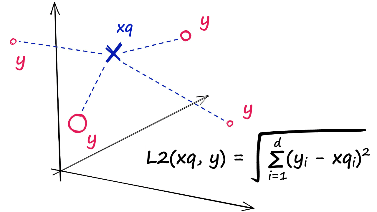
L2 distance calculation between a query vector xq and our indexed vectors (shown as y)
In Python, we would initialize our IndexFlatL2 index with our vector dimensionality (768 — the output size of our sentence embeddings) like so:
In[9]:
d = sentence_embeddings.shape[1]
d
In[10]:
index = faiss.IndexFlatL2(d)Often, we’ll be using indexes that require us to train them before loading in our data. We can check whether an index needs to be trained using the is_trained method. IndexFlatL2 is not an index that requires training, so we should return False.
Once ready, we load our embeddings and query like so:
In[5]:
index.add(sentence_embeddings)Then search given a query `xq` and number of nearest neigbors to return `k`.In[7]:
k = 4
xq = model.encode(["Someone sprints with a football"])
In[8]:
%%time
D, I = index.search(xq, k)  # search
print(I)
Out[8]:
[[4586 10252 12465  190]]
CPU times: user 27.9 ms, sys: 29.5 ms, total: 57.4 ms
Wall time: 28.9 ms
Here we're returning indices `4586`, `10252`, `12465`, and `190`, which returns:In[9]:
data['sentence_A'].iloc[[4586, 10252, 12465, 190]]Out[9]:
4586    A group of football players is running in the field
10252    A group of people playing football is running past the person
12465      Two groups of people are playing football
190    A football player is running past an official
Name: sentence_A, dtype: object
Which returns the top k vectors closest to our query vector xq as 7460, 10940, 3781, and 5747. Clearly, these are all great matches — all including either people running with a football or in the context of a football match.
Now, if we’d rather extract the numerical vectors from Faiss, we can do that too.
In[9]:
# we have 4 vectors to return (k) - so we initialize a zero array to hold them
vecs = np.zeros((k, d))
# then iterate through each ID from I and add the reconstructed vector to our zero-array
for i, val in enumerate(I[0].tolist()):
    vecs[i, :] = index.reconstruct(val)
Out[11]:
array([ 0.01627046,  0.22325929, -0.15037425, -0.30747262, -0.27122435,
       -0.10593167, -0.0646093 ,  0.04738174, -0.73349041, -0.37657705,
       -0.76762843,  0.16902871,  0.53107643,  0.51176691,  1.14415848,
       -0.08562929, -0.67240077, -0.96637076,  0.02545463, -0.21559823,
       -1.25656605, -0.82982153, -0.09825023, -0.21850856,  0.50610232,
        0.10527933,  0.50396878,  0.65242976, -1.39458692,  0.6584745 ,
       -0.21525341, -0.22487433,  0.81818348,  0.084643  , -0.76141697,
       -0.28928292, -0.09825806, -0.73046201,  0.07855812, -0.84354657,
       -0.59242058,  0.77471375, -1.20920527, -0.22757971, -1.30733597,
       -0.23081468, -1.31322539,  0.01629073, -0.97285444,  0.19308169,
        0.47424558,  1.18920875, -1.96741307, -0.70061135, -0.29638717,
        0.60533702,  0.62407452, -0.70340395, -0.86754197,  0.17673187,
       -0.1917053 , -0.02951987,  0.22623563, -0.16695444, -0.80402541,
       -0.45918915,  0.69675523, -0.24928184, -1.01478696, -0.921745  ,
       -0.33842632, -0.39296737, -0.83734828, -0.11479235,  0.46049669,
       -1.4521122 ,  0.60310453,  0.38696304, -0.04061254,  0.00453161,
        0.24117804,  0.05396278,  0.07506453,  1.05115867,  0.12383959,
       -0.71281093,  0.11722917,  0.52238214, -0.04581215,  0.26827109,
        0.8598538 , -0.3566995 , -0.64667088, -0.5435797 , -0.0431047 ,
        0.95139188, -0.15605772, -0.49625337, -0.11140176,  0.15610115])
Speed
Using the IndexFlatL2 index alone is computationally expensive, it doesn’t scale well.
When using this index, we are performing an exhaustive search — meaning we compare our query vector xq to every other vector in our index, in our case that is 14.5K L2-distance calculations for every search.
Imagine the speed of our search for datasets containing 1M, 1B, or even more vectors — and when we include several query vectors?
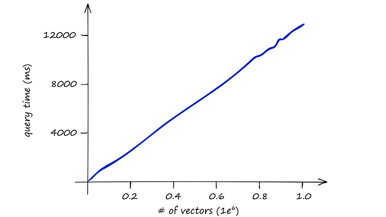
Milliseconds taken to return a result (y-axis) / number of vectors in the index (x-axis) — relying solely on IndexFlatL2 quickly becomes slow
Our index quickly becomes too slow to be useful, so we need to do something different.
Partitioning The Index
Faiss allows us to add multiple steps that can optimize our search using many different methods. A popular approach is to partition the index into Voronoi cells using an Inverted File Index (IVF) — a technique that clusters vectors during index construction, then at query time restricts the search to only the nearest cluster(s) rather than scanning every vector. This is what makes the IndexIVFFlat and IndexIVFPQ indexes so much faster than a flat exhaustive search.
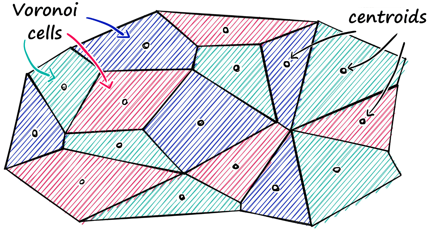
We can imagine our vectors as each being contained within a Voronoi cell — when we introduce a new query vector, we first measure its distance between centroids, then restrict our search scope to that centroid’s cell.
Using this method, we would take a query vector xq, identify the cell it belongs to, and then use our IndexFlatL2 (or another metric) to search between the query vector and all other vectors belonging to that specific cell.
So, we are reducing the scope of our search, producing an approximate answer, rather than exact (as produced through exhaustive search).
To implement this, we first initialize our index using IndexFlatL2 — but this time, we are using the L2 index as a quantizer step — which we feed into the partitioning IndexIVFFlat index.
In[12]:
nlist = 50  # how many cells
quantizer = faiss.IndexFlatL2(d)
index = faiss.IndexIVFFlat(quantizer, d, nlist)
Here we’ve added a new parameter nlist. We use nlist to specify how many partitions (Voronoi cells) we’d like our index to have.
Now, when we built the previous IndexFlatL2-only index, we didn’t need to train the index as no grouping/transformations were required to build the index. Because we added clustering with IndexIVFFlat, this is no longer the case.
So, what we do now is train our index on our data — which we must do before adding any data to the index.
In[14]:
index.train(sentence_embeddings)
index.is_trained  # check if index is now trained
In[15]:
index.add(sentence_embeddings)
index.ntotal  # number of embeddings indexed
Now that our index is trained, we add our data just as we did before.
Let’s search again using the same indexed sentence embeddings and the same query vector xq.
In[15]:
%%time
D, I = index.search(xq, k)  # search
print(I)
Out[15]:
[[ 7460 10940  3781  5747]]
CPU times: user 3.83 ms, sys: 3.25 ms, total: 7.08 ms
Wall time: 2.15 ms
The search time has clearly decreased, in this case, we don’t find any difference between results returned by our exhaustive search, and this approximate search. But, often this can be the case.
If approximate search with IndexIVFFlat returns suboptimal results, we can improve accuracy by increasing the search scope. We do this by increasing the nprobe attribute value — which defines how many nearby cells to search.
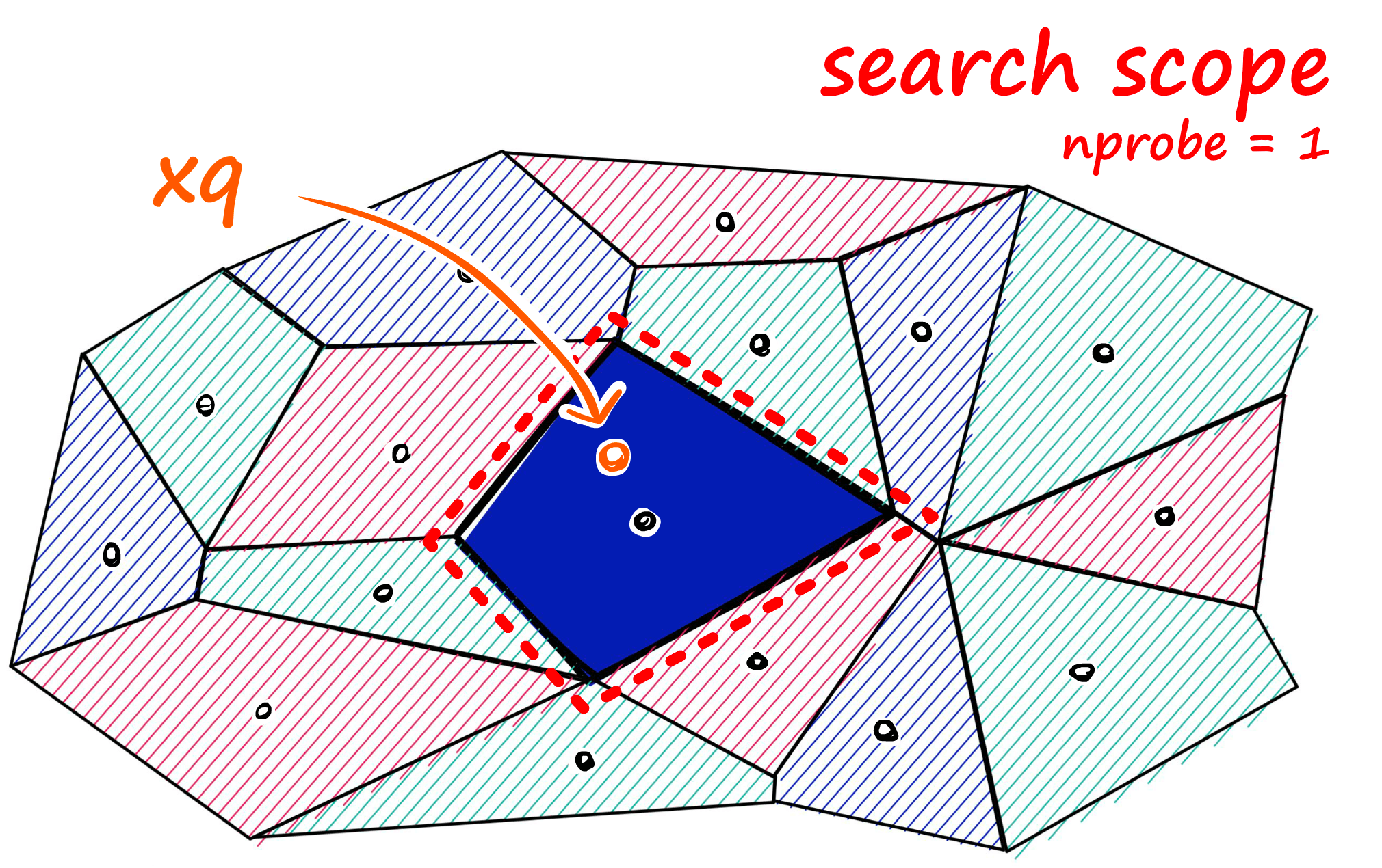
Searching the single closest cell when nprobe == 1 (left), and searching the eight closest cells when nprobe == 8 (right)
We can implement this change easily.
We can increase the number of nearby cells to search too with `nprobe`.In[17]:
%%time
D, I = index.search(xq, k)  # search
print(I)
Out[17]:
[[ 7460 10940  3781  5747]]
CPU times: user 5.29 ms, sys: 2.7 ms, total: 7.99 ms
Wall time: 1.54 ms
Now, because we’re searching a larger scope by increasing the nprobe value, we will see the search speed increase too.
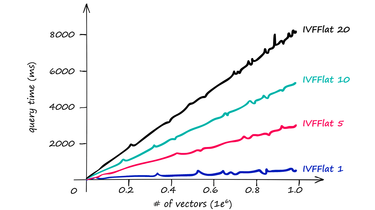
Query time / number of vectors for the IVFFlat index with different nprobe values — 1, 5, 10, and 20
Although, even with the larger nprobe value we still see much faster responses than we returned with our IndexFlatL2-only index.
Vector Reconstruction
If we go ahead and attempt to use index.reconstruct(<vector_idx>) again, we will return a RuntimeError as there is no direct mapping between the original vectors and their index position, due to the addition of the IVF step.
So, if we’d like to reconstruct the vectors, we must first create these direct mappings using index.make_direct_map().
In[20]:
index.reconstruct(7460)[:100]Out[20]:
array([ 0.01627046,  0.22325929, -0.15037425, -0.30747262, -0.27122435,
       -0.10593167, -0.0646093 ,  0.04738174, -0.7334904 , -0.37657705,
       -0.76762843,  0.16902871,  0.53107643,  0.5117669 ,  1.1441585 ,
       -0.08562929, -0.6724008 , -0.96637076,  0.02545463, -0.21559823,
       -1.256566  , -0.8298215 , -0.09825023, -0.21850856,  0.5061023 ,
        0.10527933,  0.5039688 ,  0.65242976, -1.3945869 ,  0.6584745 ,
       -0.21525341, -0.22487433,  0.8181835 ,  0.084643  , -0.761417  ,
       -0.28928292, -0.09825806, -0.730462  ,  0.07855812, -0.84354657,
       -0.5924206 ,  0.77471375, -1.2092053 , -0.22757971, -1.307336  ,
       -0.23081468, -1.3132254 ,  0.01629073, -0.97285444,  0.19308169,
        0.47424558,  1.1892087 , -1.9674131 , -0.70061135, -0.29638717,
        0.605337  ,  0.6240745 , -0.70340395, -0.86754197,  0.17673187,
       -0.1917053 , -0.02951987,  0.22623563, -0.16695444, -0.8040254 ,
       -0.45918915,  0.69675523, -0.24928184, -1.014787  , -0.921745  ,
       -0.33842632, -0.39296737, -0.8373483 , -0.11479235,  0.4604967 ,
       -1.4521122 ,  0.60310453,  0.38696304, -0.04061254,  0.00453161,
        0.24117804,  0.05396278,  0.07506453,  1.0511587 ,  0.12383959,
       -0.71281093,  0.11722917,  0.52238214, -0.04581215,  0.2682711 ,
        0.8598538 , -0.3566995 , -0.6466709 , -0.5435797 , -0.0431047 ,
        0.9513919 , -0.15605772, -0.49625337, -0.11140176,  0.15610115],
      dtype=float32)
And from there we are able to reconstruct our vectors just as we did before.
Quantization
We have one more key optimization to cover. All of our indexes so far have stored our vectors as full (eg Flat) vectors. Now, in very large datasets this can quickly become a problem.
Fortunately, Faiss comes with the ability to compress our vectors using Product Quantization (PQ).
But, what is PQ? Well, we can view it as an additional approximation step with a similar outcome to our use of IVF. Where IVF allowed us to approximate by reducing the scope of our search, PQ approximates the distance/similarity calculation instead.
PQ achieves this approximated similarity operation by compressing the vectors themselves, which consists of three steps.
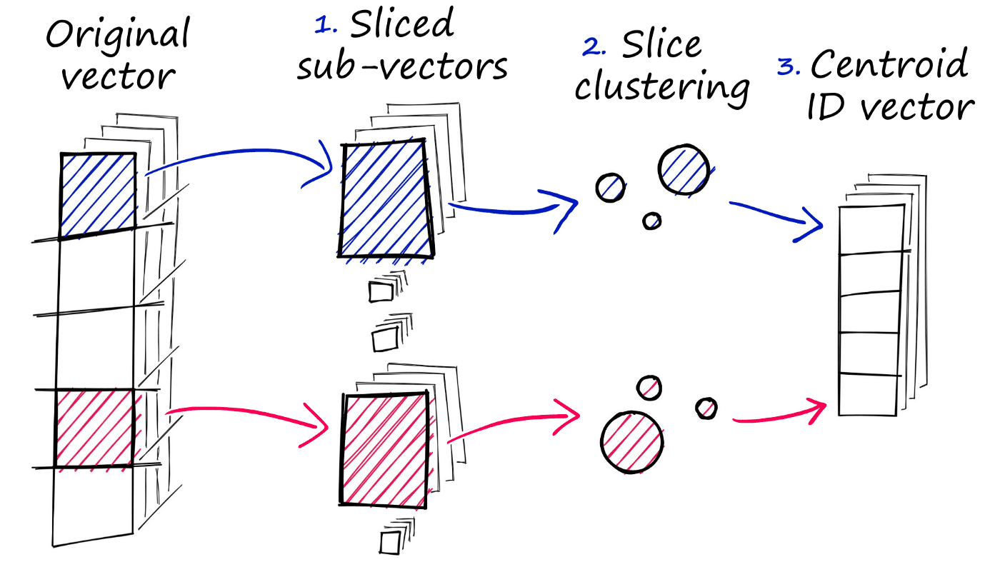
Three steps of product quantization
- We split the original vector into several subvectors.
- For each set of subvectors, we perform a clustering operation — creating multiple centroids for each sub-vector set.
- In our vector of sub-vectors, we replace each sub-vector with the ID of it’s nearest set-specific centroid.
To implement all of this, we use the IndexIVFPQ index — we’ll also need to train the index before adding our embeddings.
In[21]:
m = 8  # number of centroid IDs in final compressed vectors
bits = 8 # number of bits in each centroid

quantizer = faiss.IndexFlatL2(d)  # we keep the same L2 distance flat index
index = faiss.IndexIVFPQ(quantizer, d, nlist, m, bits)
In[23]:
index.train(sentence_embeddings)In[23]:
index.add(sentence_embeddings)And now we’re ready to begin searching using our new index.
In[24]:
index.nprobe = 10 # align to previous IndexIVFFlat nprobe valueIn[25]:
%%time
D, I = index.search(xq, k)
print(I)
Out[25]:
[[ 5013 10940  7460  5370]]
CPU times: user 3.04 ms, sys: 2.18 ms, total: 5.22 ms
Wall time: 1.33 ms
Speed or Accuracy?
Through adding PQ we’ve reduced our IVF search time from ~7.5ms to ~5ms, a small difference on a dataset of this size — but when scaled up this becomes significant quickly.
However, we should also take note of the slightly different results being returned. Beforehand, with our exhaustive L2 search, we were returning 7460, 10940, 3781, and 5747. Now, we see a slightly different order of results — and two different IDs, 5013 and 5370.
Both of our speed optimization operations, IVF and PQ, come at the cost of accuracy. Now, if we print out these results we will still find that each item is relevant:
In[26]:
[f'{i}: {sentences[i]}' for i in I[0]]Out[26]:
['5013: A group of football players running down the field.',
 '10940: A group of people playing football is running in the field',
 '7460: A group of football players is running in the field',
 '5370: A football player is running past an official carrying a football']
So, although we might not get the perfect result, we still get close — and thanks to the approximations, we get a much faster response.
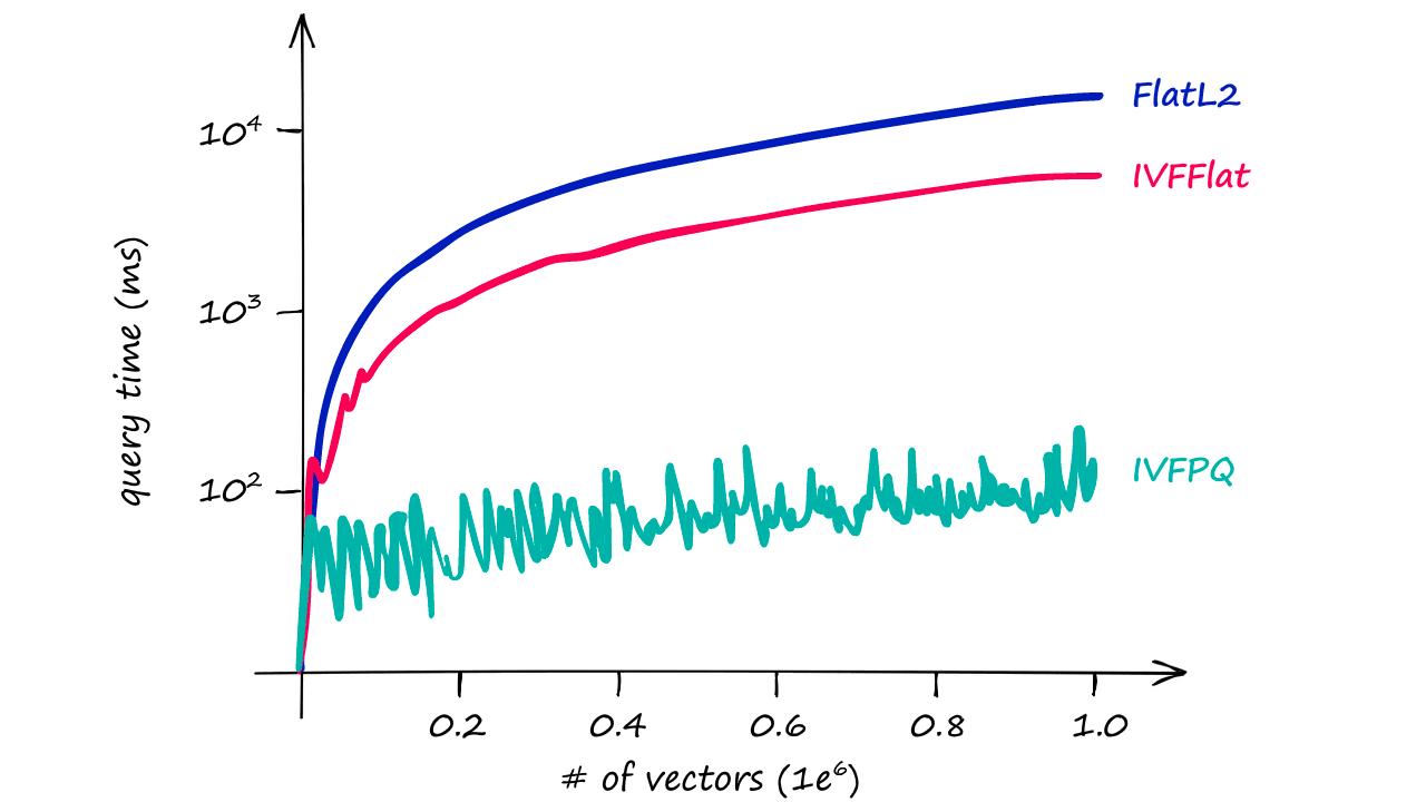
Query time / number of vectors for our three indexes
And, as shown in the graph above, the difference in query times become increasingly relevant as our index size increases.
That’s it for this article! We’ve covered the essentials to getting started with building high-performance indexes for search in Faiss.
Clearly, a lot can be done using IndexFlatL2, IndexIVFFlat, and IndexIVFPQ — and each has many parameters that can be fine-tuned to our specific accuracy/speed requirements. And as shown, we can produce some truly impressive results, at lightning-fast speeds very easily thanks to Faiss.
Want to run Faiss in production? Pinecone provides vector similarity search that’s production-ready, scalable, and fully managed.
Was this article helpful?