


Pretrained models dominate the world of machine learning. Very few ML projects begin by training a new model from scratch. Instead, people often start by taking an off-the-shelf model like Resnet or BERT and fine-tuning it for another domain, or using an existing in-house model for the same purpose.
The ecosystem of pretrained models, both external and in-house, has allowed us to push the limits of what is possible. This doesn’t mean, however, that there are no challenges.
Fortunately, we can tackle some of these problems across many different pretrained models, because they often share similar points of failure. One of those is the excessive compute and data needed to fine-tune a pretrained model for classification.
A common scenario will have some model containing a linear layer that outputs a classification. Preceding this linear layer, we can have anything from a small neural network to a billion-parameter language model. In either case, it’s the classification layer producing the final prediction.
That means we can almost ignore the preceeding model layers, and focus on the classification layer alone. This classification layer can become a single point of failure (or success) for accurate predictions.
The classification layer alone can be fine-tuned, and it often is. A common approach for fine-tuning this layer may look like this:
This approach works, but it isn’t efficient. There is a better way…
We need to focus fine-tuning efforts on essential samples that would have the greatest impact on the performance of the classifier. Otherwise, we waste time and compute by annotating and fine-tuning on samples that make little-to-no difference to model performance.
The question becomes: How do you determine which samples are essential? That’s where vector search comes in. You can use vector search to identify and focus on the essential records that really make a difference in model performance. This will save valuable time and compute by skipping all non-essential records when fine-tuning the model.
All code covering the content of this article can be found here.
Vector search will play a key role in optimizing our training steps. First, let’s understand where vector search fits into all of this.
Many state-of-the-art (SOTA) models are available for use as pretrained models. That includes models like Google’s BERT and T5, and OpenAI’s CLIP. These models use millions, even billions, of parameters and perform many complex operations. Yet, when applied to classification, these models rely on simple linear or feedforward network layers to make the final prediction.
The reason for this is that these models are not trained to make class predictions; they’re trained to make vector embeddings.
Vectors created by these models are full of helpful information that belong to a learned structure in a high-dimensional vector space. That helpful information is abstracted beyond human comprehension, but the effect is that similar items are located close to one another in vector space, whereas dissimilar items are not.
The result is that each of these models creates a “map” of information. Using this map, they can consume data, like images and text, and output a meaningful vector representation of said data.
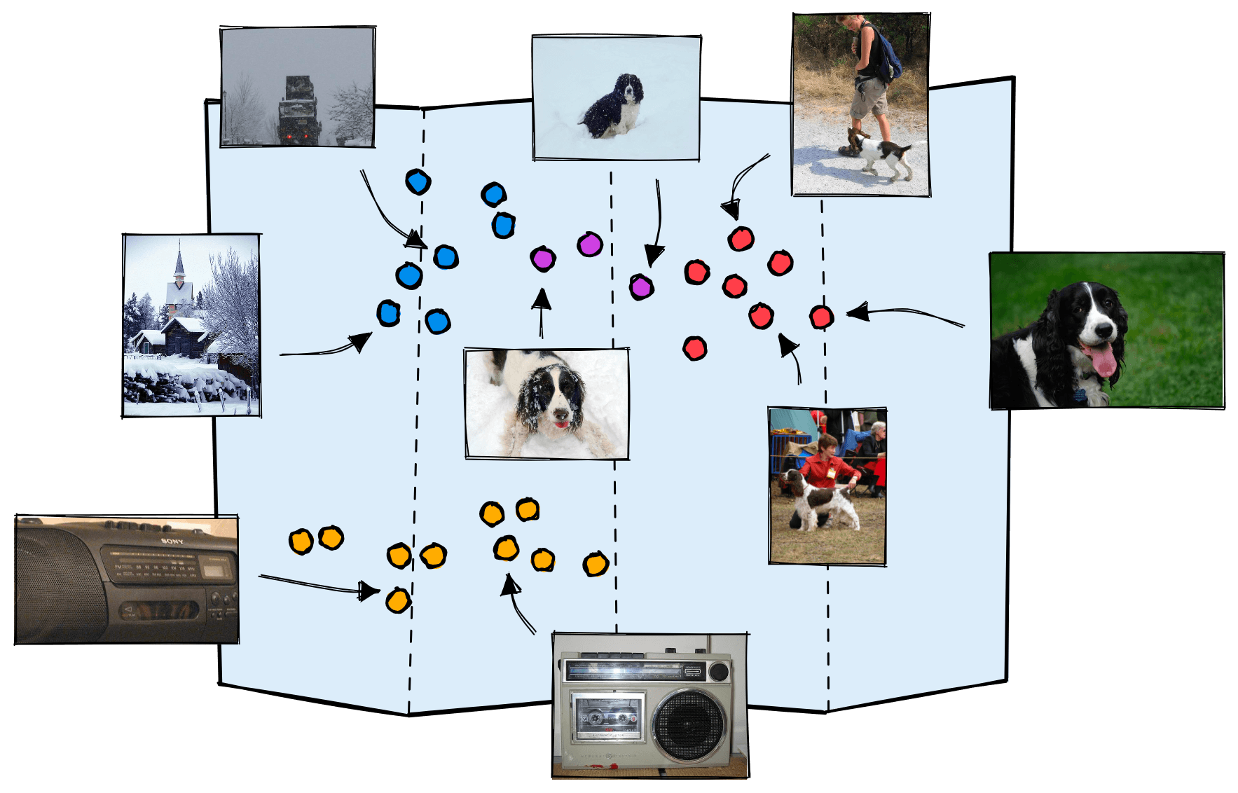
In these maps, we will find that sentences, images, or whatever form of data you’re working with belongs to a specific region based on the data’s characteristics.
Pretrained models are very good at producing accurate maps of information. Because of that, all we need to translate these into accurate class predictions is a simple layer that learns to identify the different regions in this map.
A typical architecture for classification consists of a pretrained model followed by a linear layer. A binary linear classifier (that predicts one of two labels) works by taking the dot product between an input vector and its own internal weights . Based on a threshold, the output of this operation will be categorized as one of two classes.
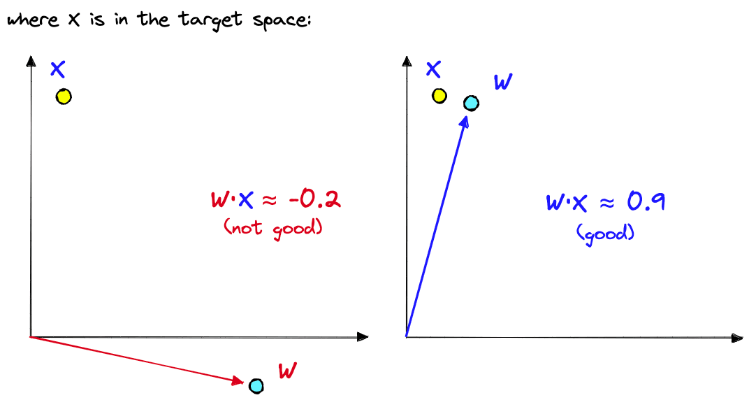
The dot product of two vectors returns a positive score if they share a similar direction, 00 if they are orthogonal, and a negative score if they have opposite directions.
There is one key problem with dot product similarity, it considers both direction and magnitude. Magnitude is troublesome because vectors with greater magnitudes often overpower more similar, lower-magnitude vectors. To avoid this, we normalize the vectors being output by our pretrained models.
The result is that a linear classifier must learn to align its internal weights with the vectors labeled as and push its internal weights away from vectors labeled as .
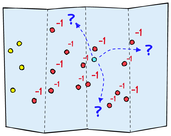
Fine-tuning the classifier like this works, but there are some unecessary limitations. First, imagine we return only irrelevant samples for a training batch. They will all be marked as . The classifier knows to move away from these values but it cannot know which direction to move towards. In high-dimensional spaces, this is problematic and will cause the classifier to move at random.
Second, many training samples may be more or less relevant. “A dog” is more relevant than “a truck” to the query “dogs in the snow”, yet, “a dog in the snow” is not equally relevant as “a dog”.
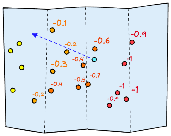
What we need is a gradient of relevance, a continuous range from -1 to +1. The first problem is solved as the range of scores gives the classifier information on the best direction of movement. And the second problem is solved as we can now be more precise with our relevance scores.
All of this allows a linear classifier to learn where to place itself within the vector space produced by the model layers preceding it.
That describes the fine-tuning process, but we cannot do this across our entire dataset. It would take too much time annotating everything. To do this efficiently, we must capitalize on the idea of identifying relevant vs. irrelevant vectors within proximity of the model’s learned weights.
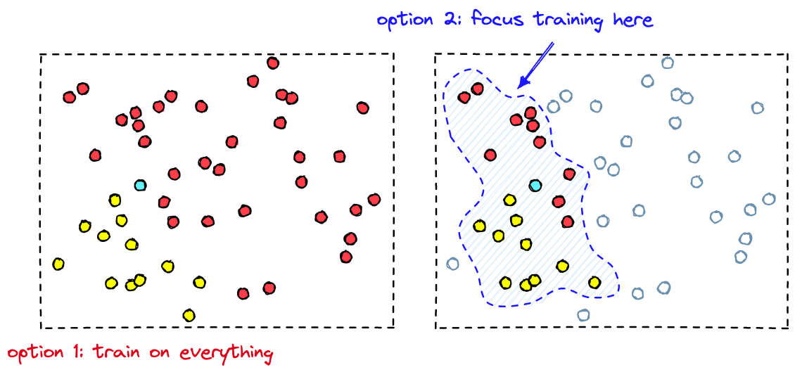
By identifying the vectors with the highest proximity to the classifier’s learned boundaries, we are able to skip irrelevant samples that make little-to-no impact on the classifier performance. Instead, we hone-in on the critical area of vectors near the target vector space.
During training, we need to feed vectors generated by the preceding layers into our linear classifier. Those vectors also need to be labeled. But, if our classifier is already tuned to understand the vector space generated by the previous layers, most training data is unlikely to be helpful.
We need to focus our fine-tuning efforts on records that are similar enough to our target class to confuse our model. For an already trained classifier, these are the false positives and false negatives predicted by the classifier.
However, we don’t usually have a list of false positives and false negatives. But we do know that the solvable errors will be present near the classifiers decision boundary; the line that separates the positive predictions from negative predictions.
Due to the proximity of these samples, it is harder for the classifier to find the exact boundary that best identifies true positives vs. true negatives.
Vector search allows us to retrieve the high proximity samples most similar to the model weights . We can then label the returned samples and use them for training our model. The model optimizes its internal weights; we extract them again, search, and repeat.
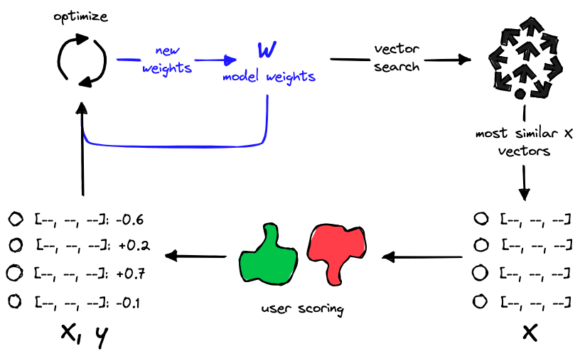
We focus annotation and training on essential samples by retrieving the most similar vectors. Doing this avoids wasting time and compute on samples that make little to no difference to our model performance.
Now let’s combine all this to fine-tune a linear classifier with vector search.
There are two parts to our training process:
If you already have an indexed dataset, you can skip ahead to the Fine-tuning section. If not, we’ll work through the indexing steps next.
Given a dataset of images (or other formats), we first need to process everything through the preceding model layers to generate a list of vectors to be indexed. These vectors will later be used as the training data for the model.
The terms vectors, embeddings, and vector embeddings will be used interchangeably. When specifying embeddings produced by a specific medium (such as images or text), we will refer to them as “image embeddings” or “text embeddings”.
For our example, we will use a model capable of comparing both text and images called CLIP. OpenAI’s CLIP has been trained to match similar natural language prompts to images. It does this by encoding pairs as closely as possible in a vector space.
We need an image dataset and CLIP (swap these for your dataset and model where relevant). We will use the frgfm/imagenette dataset found on Hugging Face datasets.
In the “image” feature of the dataset, we have ~9.4K images of various sizes stored as PIL objects. Inside a Jupyter notebook, we can view them like so:
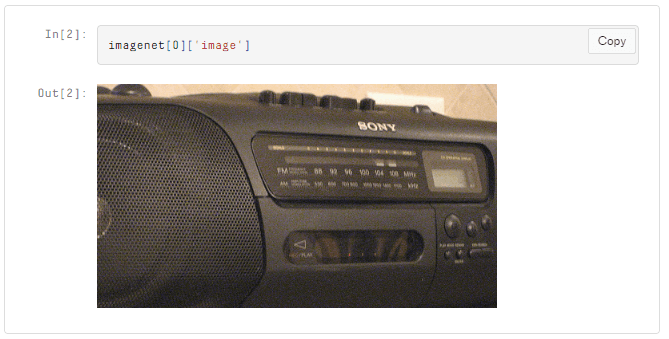
We embed these images using CLIP, which we initialize through the HuggingFace Transformers library.
# !pip install transformers torch
from transformers import CLIPProcessor, CLIPModel
import torch

device = "cuda" if torch.cuda.is_available() else "cpu"

model_id = "openai/clip-vit-base-patch32"
model = CLIPModel.from_pretrained(model_id).to(device)
processor = CLIPProcessor.from_pretrained(model_id)
We can embed an image and transform it into a flat Python list (ready for indexing) like so:
The later linear classifier uses dot product to calculate predictions. That means we must also use dot product to measure the similarity between image embeddings during the vector search. Given two similar images of dogs and an image of a radio, we would expect the two dog images to return a higher score.
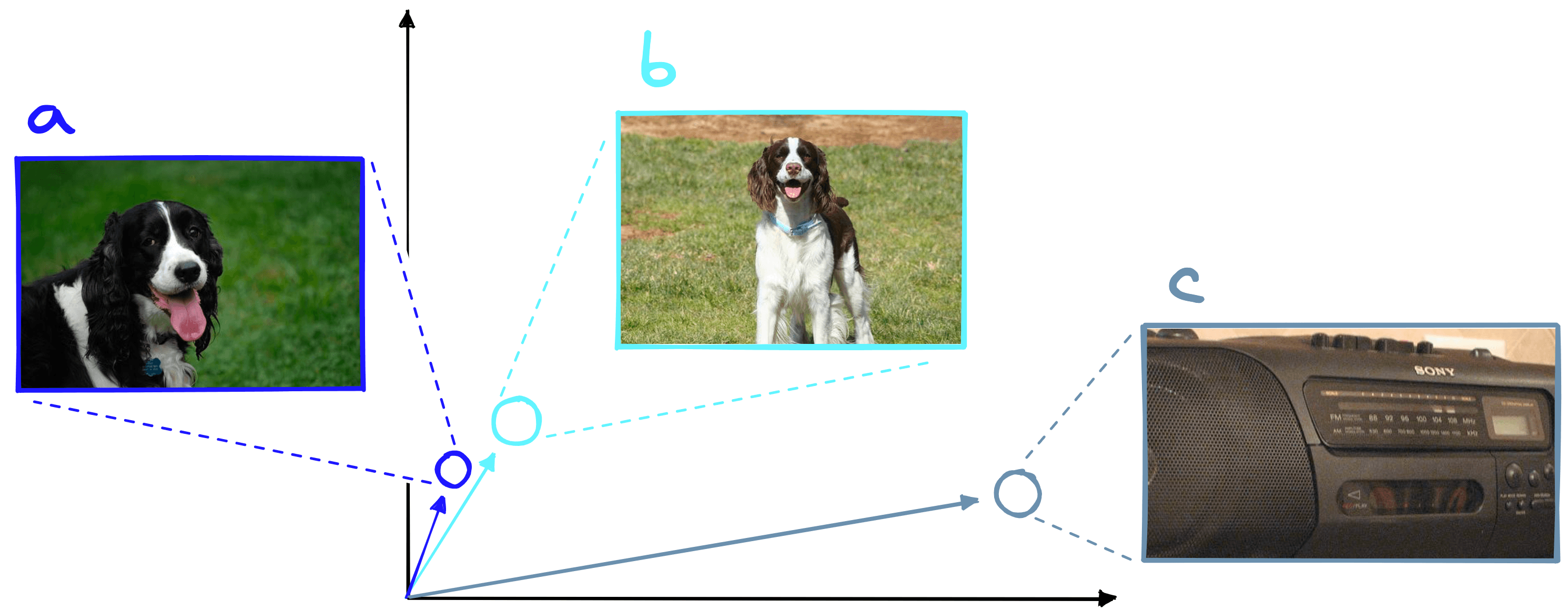
We would expect two nearby embeddings like a and b to return a higher similarity score than with c. Yet, when we calculate the dot product between these embeddings, the magnitude of c outputs a higher output.
Dot product is heavily influenced by vector magnitude. This means two very similar vectors with low magnitude can score lower than if they were compared to a dissimilar vector with greater magnitude.
We solve this problem by normalizing all of our vectors beforehand. By doing this, we “flatten” the magnitude across vectors, leaving just the angular difference between them.
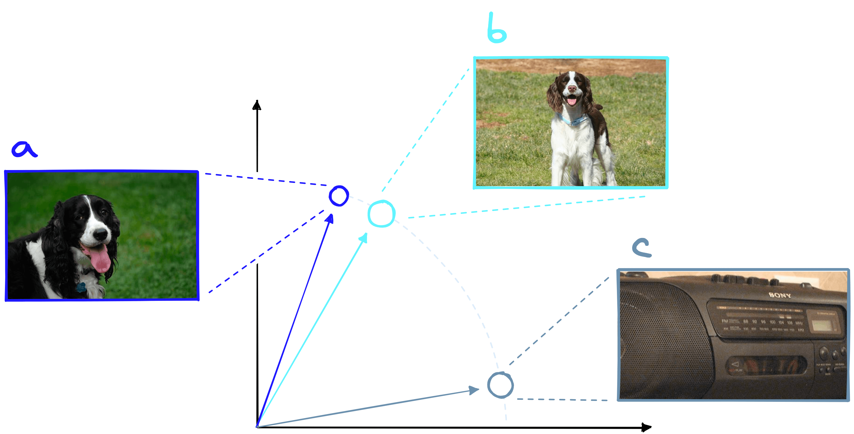
Normalization “flattens” the magnitude of our vectors.
After normalization of our embedding with emb = emb / np.linalg.norm(emb), we can move on to indexing it in our vector database.
Here we will use the Pinecone vector database. All we need is a free API key and environment variable that can be found here. To install the Pinecone Python client, we use pip install pinecone-client. Finally, we import and initialize the connection.
import pinecone

pinecone.init(api_key="YOUR_API_KEY", environment="YOUR_ENV")
# (default env is 'us-east1-gcp')
After connecting to Pinecone, we create a new index where we will store our vectors.
index_name = "imagenet-query-trainer-clip"

pinecone.create_index(
    index_name,
    dimension=emb.shape[0],
    metric="dotproduct",
    metadata_config={"indexed": ["seen"]}
)
# connect to the index
index = pinecone.Index(index_name)
We specify four parameters for our index:
index_name: The name of our vector index, it can be anything.dimensions: The dimensionality of our vector embeddings. This must match the vector dimensionality output by CLIP. All future vectors must have the same dimensionality. Our vectors have 768 dimensions.metric: This is the similarity metric we will use. Pinecone accepts "euclidean", "cosine", and "dotproduct". As discussed, we will be using "dotproduct".metadata_config: Pinecone has both indexed and non-indexed metadata. Indexed metadata can be used in metadata filtering, and we need this for " exploring “ the image dataset. So, we index a single field called "seen".With this, we have indexed a single vector (emb) in our Pinecone index. We can check this by running index.describe_index_stats() which will return:
{'dimension': 512,
'index_fullness': 0.0,
'namespaces': {'': {'vector_count': 1}},
'totalVectorCount': 1.0}
Those are all the steps we need to embed and index an image. Let’s apply these steps to the remainder of the dataset.
There’s little we can do with a single vector, so we will repeat the previous steps on the rest of our dataset. We place the previous logic into a loop, iterate once over the dataset, and we’re done.
from tqdm.auto import tqdm
batch_size = 64

for i in tqdm(range(0, len(imagenet), batch_size)):
    # select the batch start and end
    i_end = min(i + batch_size, len(imagenet))
    # some images are grayscale (mode=='L') we only keep 'RGB' images
    images = [img for img in imagenet[i:i_end]['image'] if img.mode == 'RGB']
    # process images and extract pytorch tensor pixel values
    image = processor(
        text=None,
        images=images,
        return_tensors='pt',
        padding=True
    )['pixel_values'].to(device)
    # feed tensors to model and extract image features
    out = model.get_image_features(pixel_values=image)
    out = out.squeeze(0)
    # take the mean across each dimension to create a single vector embedding
    embeds = out.cpu().detach().numpy()
    # normalize and convert to list
    embeds = embeds / np.linalg.norm(embeds, axis=0)
    embeds = embeds.tolist()
    # create ID values
    ids = [str(i) for i in range(i, i_end)]
    # prep metadata
    meta = [{'seen': 0} for image in images]
    # zip all data together and upsert
    to_upsert = zip(ids, embeds, meta)
    index.upsert(to_upsert)
There’s a lot of code here, but it’s nothing more than a compact version of the previous steps. We can check the number of records added using the describe_index_stats method.
{'dimension': 512,
'index_fullness': 0.0,
'namespaces': {'': {'vector_count': 9296}},
'totalVectorCount': 9296.0}
We have slightly fewer records here because we drop grayscale images in the upsert loop (line 8).
With everything indexed, we’re ready to take our classifier model and optimize it on the most relevant samples in our dataset. You can follow along live using this Colab notebook.
You may or may not have a classifier already trained. If you do have a classifier, you can skip ahead a few paragraphs to the Classifier section.
If you do not have a classifier, we can begin by setting the model weights equal to the vector produced by a relevant query. This is where the text-to-image capabilities of CLIP come into use. Given a natural language prompt like “dogs in the snow”, we can use CLIP to embed this into the same vector space as our image embeddings.
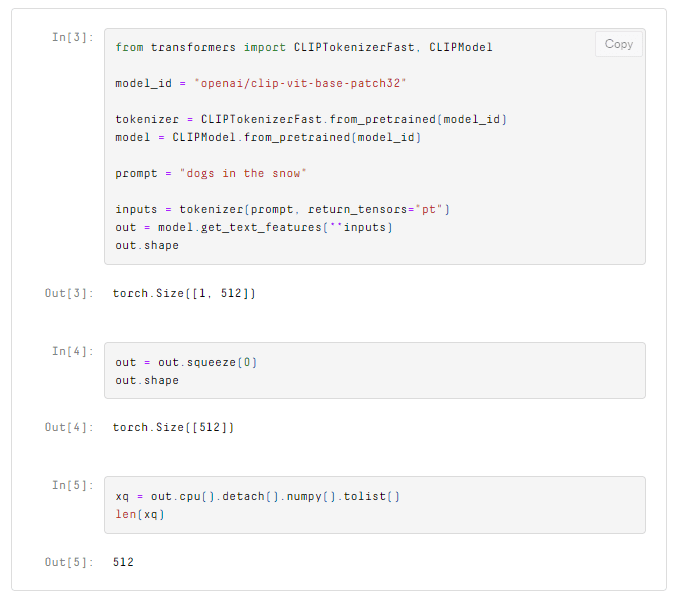
We will set our initial model weights equal to xq, but first, let’s retrieve the first batch of training samples.
As with the image embeddings, we need to transform the CLIP output into a flat list for querying with Pinecone and retrieving the image idx and vector values:
xc = index.query(xq, top_k=10, include_values=True)

# get the index values
idx = [int(match['id']) for match in xc['matches']]
# get the vectors
values = [match['values'] for match in xc['matches']]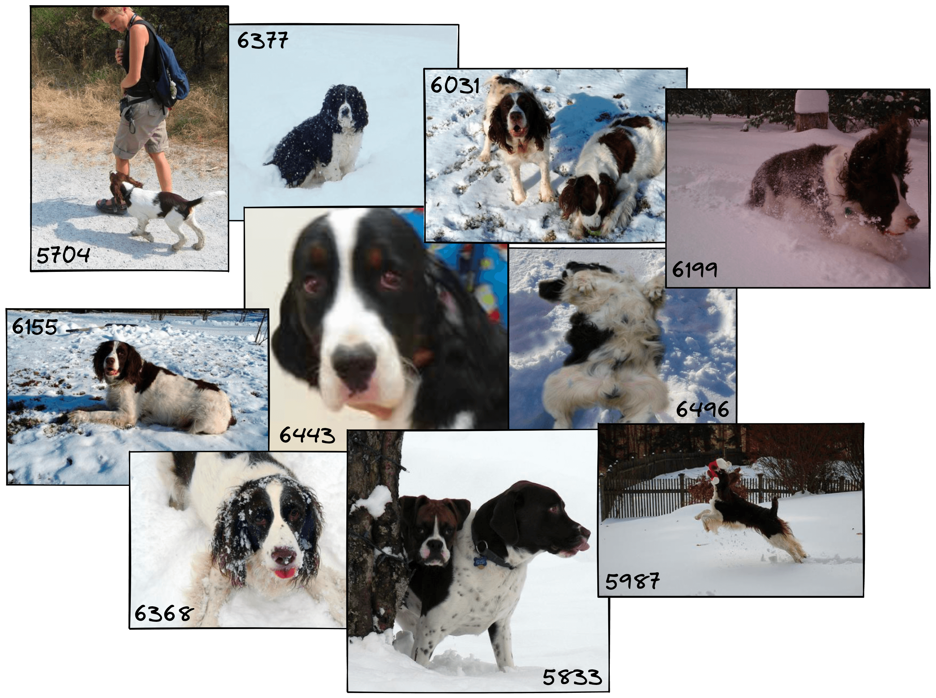
The “dogs in the snow” query is mostly accurate, with the two exceptions showing dogs on non-snow yet white backgrounds.
These images and their embeddings act as the training data for our classifier. The embeddings themselves will become the inputs X. We allow the user to create the labels y by entering a score from -1 to +1. All of this will be performed by a function called score_images, the code for this can be found here.
Above we can see the images followed by a printout of their ID values and the scores assigned to them, all of these pairs are stored in scores as a dictionary. These scores are our training data; all that is left is to train our model with it. So, we initialize the classifier.
Here, we will use a simple linear binary classifier in PyTorch. The model weights will act as our future query vectors. As the model learns to distinguish between relevant and irrelevant vectors, it will optimize its internal weights to produce a vector more like the vectors we marked with the label 1 (relevant).
import torch

# initialize the model with 512 input size (equal to vector size) and one output
model = torch.nn.Linear(512, 1)

# convert initial query `xq` to tensor paramater for initial model weights
init_weight = torch.Tensor(xq).reshape(1, -1)
model.weight = torch.nn.Parameter(init_weight)

# init loss and optimizer
loss = torch.nn.BCEWithLogitsLoss()
# we set the lr high for these examples, in real-world use case this
# may need to be lower for more stable fine-tuning
optimizer = torch.optim.SGD(model.parameters(), lr=0.2)
On lines 7-8, we set the model weights to the initial query we made. If you already have a classifier, this part is not necessary. By initializing the model weights like this, we start in a more relevant vector space, from which we can begin fine-tuning the model and optimizing our query.
We will write a small PyTorch training loop and place it in a function called fit. The number of iterations iters can be set to move slower/faster through the vector space for each training batch.
model.train()  # switch model to training mode

def fit(X: list, y: list, iters: int = 5):
    for _ in range(iters):
        # get predictions
        out = model(torch.Tensor(X))
        # calculate loss
        loss_value = loss(out, torch.Tensor(y).reshape(-1, 1))
        # reset gradients
        optimizer.zero_grad()
        # backpropagate
        loss_value.backward()
        # update weights
        optimizer.step()

# train
fit(X, y)
After we’ve run the training loop, we can extract the new model weights to use as our next query vector, xq.
xq = model.weight.detach().numpy()[0].tolist()We can return many of the same items during training if querying with this slightly fine-tuned xq vector. Increasing lr and iters to shift the fine-tuned xq values more quickly might avoid this, but it will struggle to converge on an optimal query. On the other hand, decreasing lr and iters will mean we keep seeing the same set of images and will overfit them.
We want the classifier to see a broader range of both positive and negative images without needing excessive values for lr and iters. Instead, we keep these two parameters low and filter out all previously seen images.
These examples use excessively high lr and iters parameters to demonstrate the movement across vector space. We recommended using lower values to provide a more stable training process.
Filtering is done via Pinecone’s metadata filtering. Earlier we initialized the index with metadata_config={"indexed": ["seen"]} and added {"seen": 0} to the metadata of every record. All of that was for this next step. We set their metadata for the previous 10 retrieved records to {"seen": 1}.
# we must update one record at a time
for i in idx:
    index.update(str(i), set_metadata={"seen": 1})
When we query again, we can add a filter condition filter={"seen": 0} to return only unseen records.
# retrieve most similar records
xc = index.query(
    xq,
    top_k=10,
    include_values=True,
    filter={"seen": 0}
)
# extract index and vector values
idx = [int(match['id']) for match in xc['matches']]
values = [match['values'] for match in xc['matches']]
Starting with dogs in the snow, let’s imagine we’d like to adjust our already well-trained “dogs in snow” classifier to become a “dogs at dog shows” classifier. How do we influence the model to retrieve images from this new domain?
Traversing across clusters of similar images in the semantic query trainer app, this example uses irrelevant/relevant labels. The app has since been updated to use contrastive sliders to score images.
The example above starts with our slightly fine-tuned “dogs in the snow” embedding in both windows. We then change what is marked as relevant. The left window shows us traversing from dogs in the snow to garbage trucks and back to dogs. In the right window, we traverse to dogs in fields and finally to dog shows.
We can replicate this process by repeating the logic we have already worked through. You can find an example that wraps this code into a few training/retrieval functions here.
As we keep doing this, the number of retrieved dog images will quickly increase until they dominate the returned images, or we simply exhaust all relevant images. At this point, we can stop and test our newly trained query vector on the unfiltered dataset. We can do this in one of two ways:
filter argument in query. This is ideal if performing a quick test but will not work if planning to perform a second loop through the dataset or train another query.{"seen": 1} back to {"seen": 0}.To apply method 2, we iteratively query the index with a filter of {"seen": 1}, resetting the metadata, and stop only when we return no more records.
while True:
    xc = index.query(xq, top_k=100, filter={"seen": 1})
    idx = [match['id'] for match in xc['matches']]
    if len(idx) == 0: break
    for i in idx:
        index.update(str(i), set_metadata={"seen": 0})
When we search again, we will return a completely unfiltered view of the search results.
xc = index.query(
    xq,
    top_k=10
)
# extract index and vector values
idx = [int(match['id']) for match in xc['matches']]

# show the results
for i in idx:
    print(i)
    plt.imshow(imagenet[i]['image'])
    plt.show()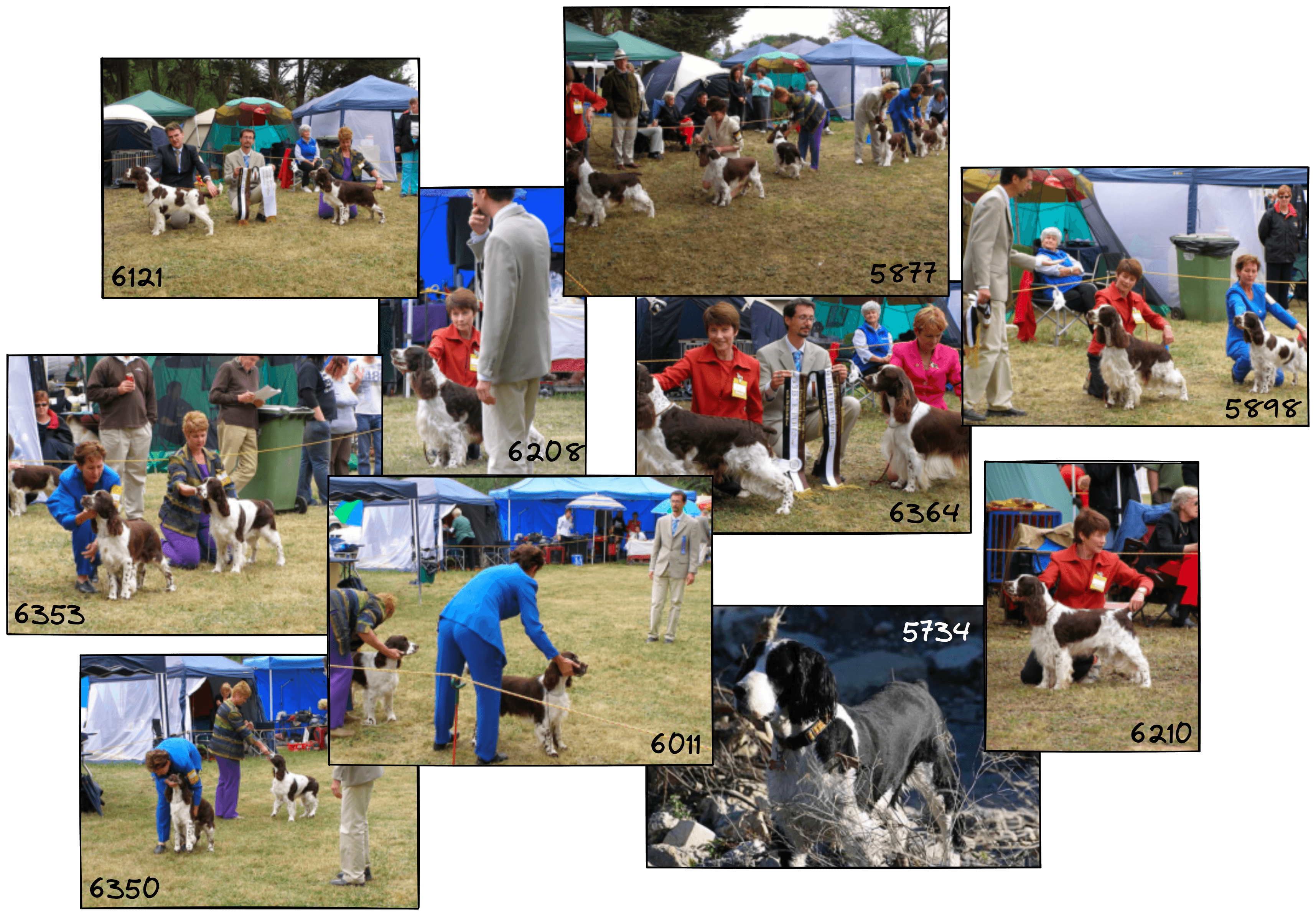
Images retrieved after fine-tuning the query for retrieving dog shows.
Our query has clearly been optimized for finding images of dog shows. We can go ahead and save our classifier model.
with open("classifier.pth", "wb") as f:
    torch.save(model, f)
In the next section, we’ll look at classifying images using our model fine-tuned with vector search.
We know how to optimize our query and hone in on specific concepts and clusters of images. With this, our classifier has hopefully become great at identifying images of dog shows. Its internal weights should have aligned to the vectors that best represent the concept of “dog shows”.
There is just one more step. How do we make and interpret predictions with our new classifier? We start by loading the classifier from file (you can skip the save/load if preferred and use the same instance).
with open("classifier.pth", "rb") as f:
    clf = torch.load(f)
We will test the predictions on the validation split of the imagenette dataset. To download this, we run the same load_dataset function as before but change the split parameter to validation.
imagenet = load_dataset(
    'frgfm/imagenette',
    'full_size',
    split='validation',  # here we switch to validation set
    ignore_verifications=False  # set to True if seeing splits Error
)
Let’s start with a dog show image and see what model outputs. As before, we will process and create the image embedding using CLIP.
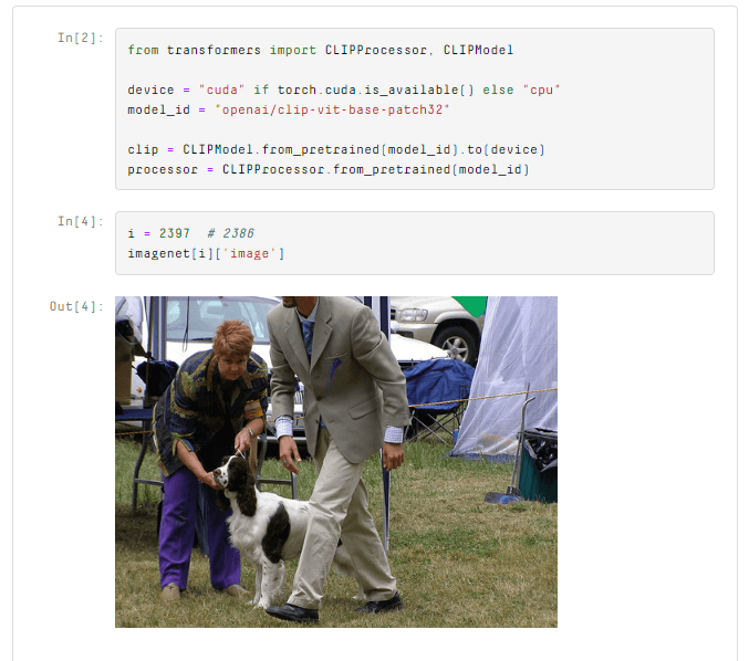
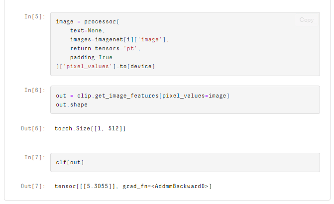
The prediction is positive, meaning the model predicts an image of a dog show! Let’s try another.
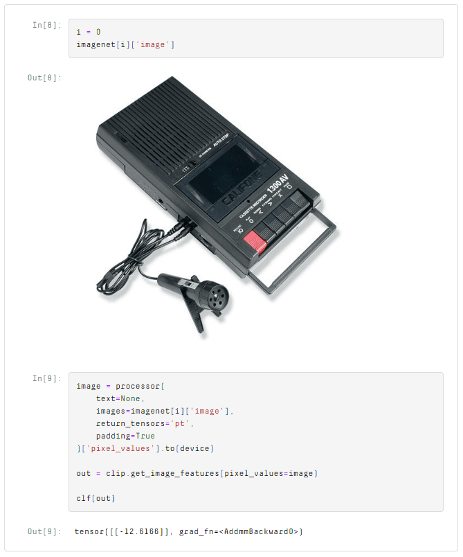
A negative value means the model predicts this is not a dog show. We can use this same logic to make predictions for the complete validation set and look at what the model predicts as dog shows.
from tqdm.auto import tqdm

batch_size = 64

preds = []

for i in tqdm(range(0, len(imagenet), batch_size)):
    i_end = min(i+batch_size, len(imagenet))
    image = processor(
        text=None,
        images=imagenet[i:i_end]['image'],
        return_tensors='pt',
        padding=True
    )['pixel_values'].to(device)
    out = clip.get_image_features(pixel_values=image)
    logits = clf(out)
    preds.extend(logits.detach().cpu().numpy().reshape(1, -1)[0].tolist())
We add these predictions to our dataset, filter out any results where the prediction is negative, and then sort the results.
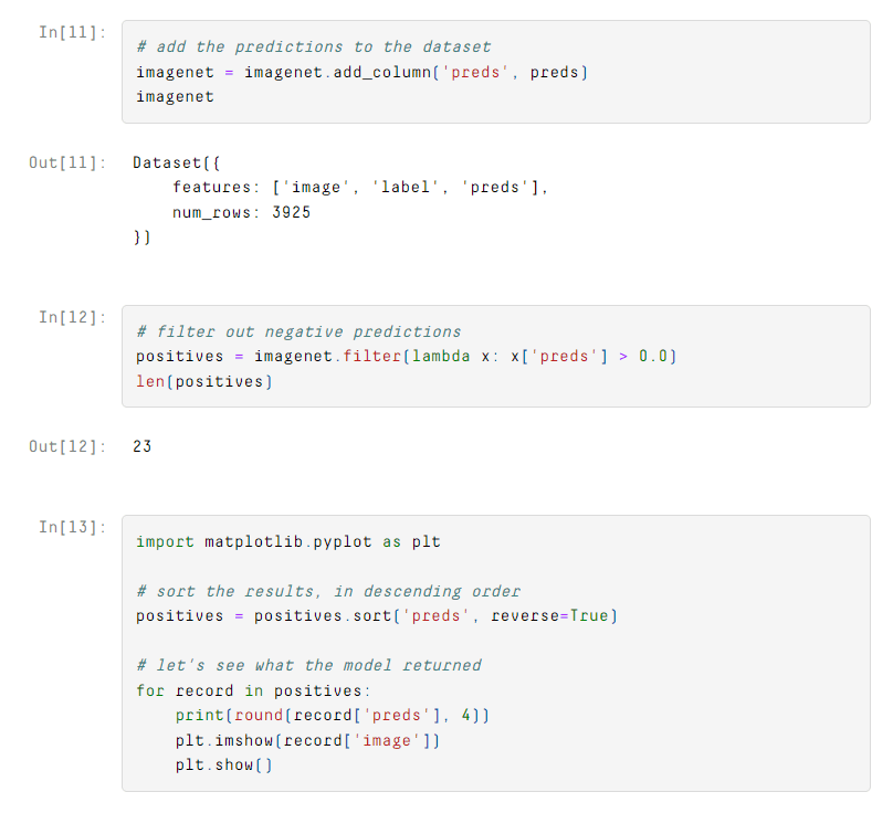
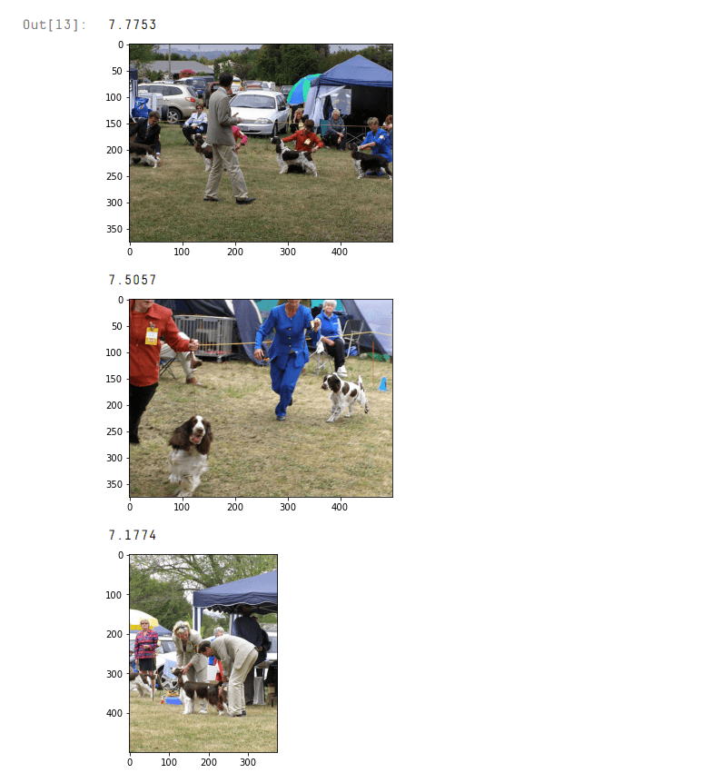
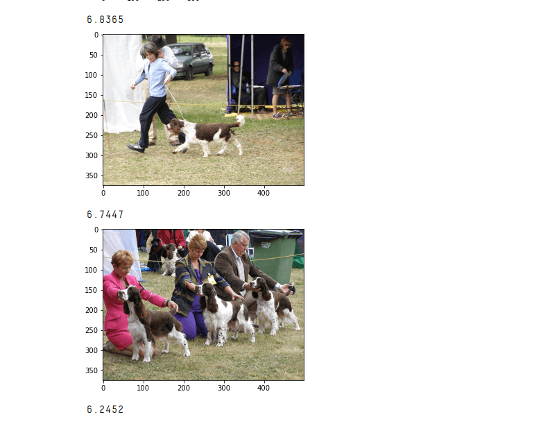
These look like great results. There are 23 results in total, and all but two of them are images of dog shows (find the complete set of results here.
That is how we can optimize fine-tuning for linear classification layers with vector search. With this, we can hone in on what is important for our classifier and focus on these critical samples rather than slogging through the entire dataset and fine-tuning the model at random.
Doing this for an image classifier is just one example. We can apply this to various use cases, from anomaly detection to recommendation engines. The pool of use cases involving vector search is growing daily.
此内容由惯性聚合(RSS阅读器)自动聚合整理,仅供阅读参考。 原文来自 — 版权归原作者所有。