


Browsing, searching, and retrieving images has never been easy. Traditionally, many technologies relied on manually appending metadata to images and searching via this metadata. This approach works for datasets with high-quality annotation, but most datasets are too large for manual annotation.
That means any large image dataset must rely on Content-Based Image Retrieval (CBIR). Search with CBIR focuses on comparing the content of an image rather than its metadata. Content can be color, shapes, textures – or with some of the latest advances in ML — the “semantic meaning” behind an image.
Color histograms represent one of the first CBIR techniques, allowing us to search through images based on their color profiles rather than metadata.
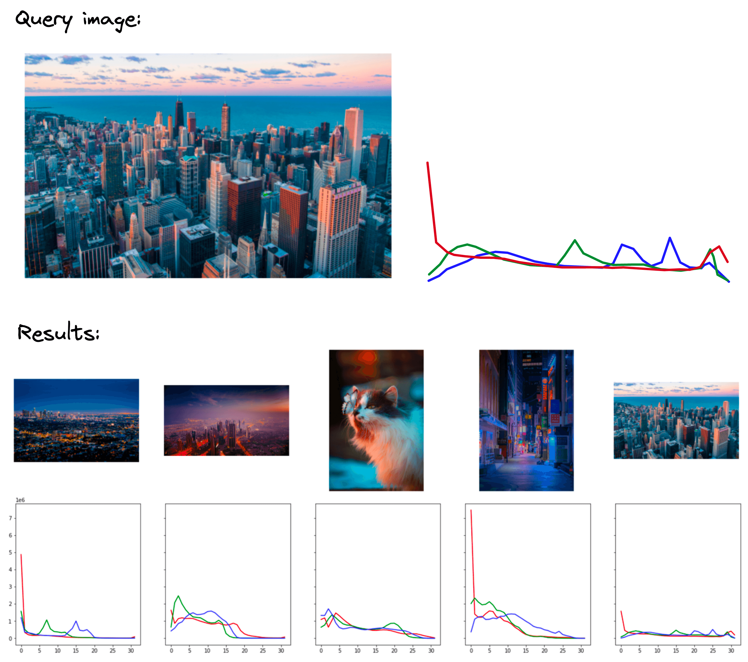
Using the top query image we return the top five most similar images (including the same image) based on their color profiles.
These examples demonstrate the core idea of color histograms. That is, we take an image, translate it into color-based histograms, and use these histograms to retrieve images with similar color profiles.
There are many pros and cons to this technique, as we will outline later. For now, be aware that this is a one of the earliest methods for CBIR, and many newer methods may be more useful (particularly for more advanced use-cases). Let’s begin by focusing on understanding color histograms and how we can implement them in Python.
The original code notebooks covering the content of this article can be found here.
Color Histograms
To create our histograms we first need images. Feel free to use any images you like, but, if you’d like to follow along with the same images, you can download them using HuggingFace Datasets.
from datasets import load_dataset  # !pip install datasets

data = load_dataset('pinecone/image-set', split='train', revision='e7d39fc')
Inside the image_bytes feature of this dataset we have base64 encoded representations of 21 images. We decode them into OpenCV compatible Numpy arrays like so:
from base64 import b64decode
import cv2
import numpy as np

def process_fn(sample):
    image_bytes = b64decode(sample['image_bytes'])
    image = cv2.imdecode(np.frombuffer(image_bytes, np.uint8), cv2.IMREAD_COLOR)
    return image

images = [process_fn(sample) for sample in data]
This code leaves us with the images in the list images. We can display them with matplotlib.
The three dogs look strangely blue; that’s not intentional. OpenCV loads images in a Blue Green Red (BGR) format. Matplotlib expected RGB, so we must flip the color channels of the array to get the true color image.
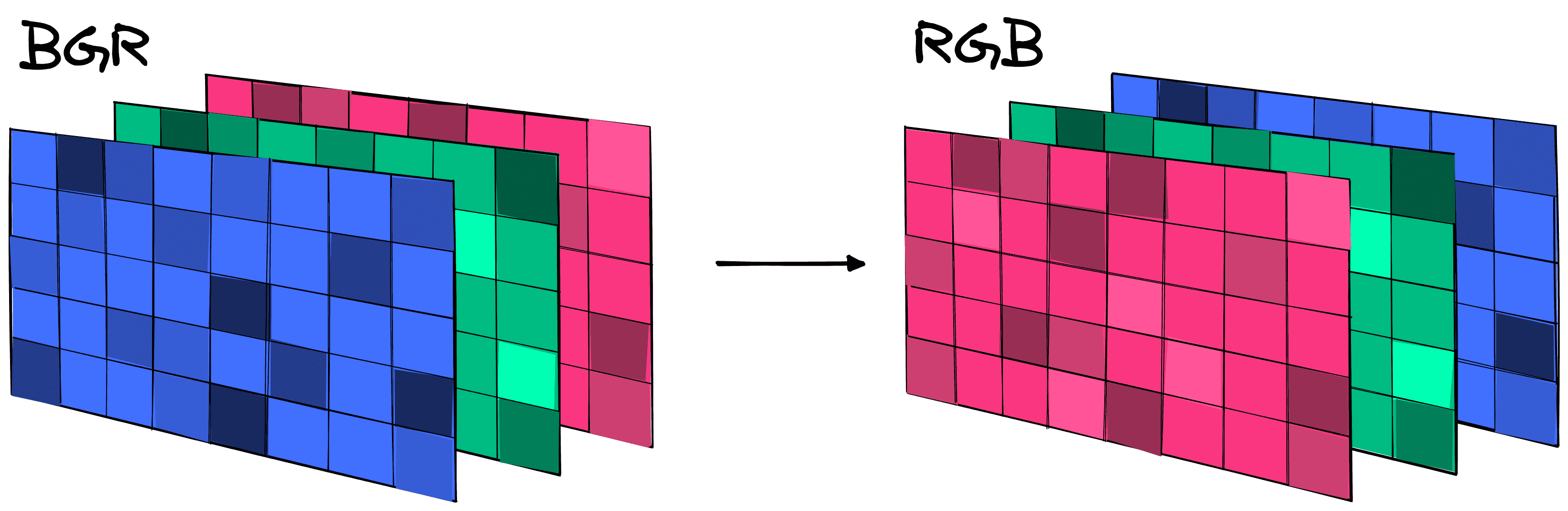
OpenCV reads images using BGR format, we flip the arrays to RGB so that we can view the true color image in matplotlib.
Note that while the shape of the array has remained the same, the three values have reversed order. Those three values are the BGR-to-RGB channel values for a single pixel in the image. As shown, after flipping the order of these channels, we can display the true color image.
Just want to create some color histogram embeddings? Skip ahead to the OpenCV Color Histograms section!
Step-by-Step with Numpy
To help us understand how an image is transformed into a color histogram we will work through a step-by-step example using Numpy. We already have our Numpy arrays. For the first image we can see the three BGR color values at pixel zero with:
[Out]: array([165, 174, 134], dtype=uint8)
Every pixel in each image has three BGR color values like this that range on a scale of 0 (no color) to 255 (max color). Using this, we can manually create RGB arrays to display colors with Matplotlib like so:
From the first pixel of our image with the three dogs, we have the BGR values:
We can estimate that this pixel will be a relatively neutral green-blue color, as both of these colors slightly overpower red. We will see this color by visualizing that pixel with matplotlib:
The color channel values for all pixels in the image are presently stored in an array of equal dimensions to the original image. When comparing image embeddings the most efficient techniques rely on comparing vectors not arrays. To handle this, we first reshape the rows and columns of the image array into a single row.
image_vector = rgb_image.reshape(1, -1, 3)
image_vector.shape
[Out]: (1, 4096000, 3)
We can see that the top left three pixels are still the same:
Even now, we still don’t have a “vector” because there are three color channels. We must extract those into their own vectors (and later during comparison we will concatenate them to form a single vector).
red = image_vector[0, :, 0]
green = image_vector[0, :, 1]
blue = image_vector[0, :, 2]

red.shape, green.shape, blue.shape
[Out]: ((4096000,), (4096000,), (4096000,))
Now we visualize each with a histogram.
Here we can see the three color channels RGB. On the x-axis we have the pixel color value from 0 to 255 and, on the y-axis, is a count of the number of pixels with that color value.
Typically, we would discretize the histograms into a smaller number of bins. We will add this to a function called build_histogram that will take our image array image and a number of bins and build a histogram for us.
def build_histogram(image, bins=256):
    # convert from BGR to RGB
    rgb_image = np.flip(image, 2)
    # show the image
    plt.imshow(rgb_image)
    # convert to a vector
    image_vector = rgb_image.reshape(1, -1, 3)
    # break into given number of bins
    div = 256 / bins
    bins_vector = (image_vector / div).astype(int)
    # get the red, green, and blue channels
    red = bins_vector[0, :, 0]
    green = bins_vector[0, :, 1]
    blue = bins_vector[0, :, 2]
    # build the histograms and display
    fig, axs = plt.subplots(1, 3, figsize=(15, 4), sharey=True)
    axs[0].hist(red, bins=bins, color='r')
    axs[1].hist(green, bins=bins, color='g')
    axs[2].hist(blue, bins=bins, color='b')
    plt.show()
We can apply this to a few images to get an idea of how the color profile of an image can change the histograms.
That demonstrates color histograms and how we build them. However, there is a better way.
OpenCV Histograms
Building histograms can be abstracted to be done more easily using the OpenCV library. OpenCV has a function called calcHist specifically for building histograms. We apply it like so:
red_hist = cv2.calcHist(
    [images[5]], [2], None, [64], [0, 256]
)
green_hist = cv2.calcHist(
    [images[5]], [1], None, [64], [0, 256]
)
blue_hist = cv2.calcHist(
    [images[5]], [0], None, [64], [0, 256]
)

red_hist.shape
[Out]: [64, 1]
The values used here are:
cv2.calcHist(
 [images], [channels], [mask], [bins], [hist_range]
)
Where:
imagesis our cv2 loaded image with a BGR color channel. This argument expects a list of images which is why we have placed a single image inside square brackets[].channelsis the color channel (BGR) that we’d like to create a histogram for; we do this for a single channel at a time.maskis another image array consisting of0and1values that allow us to mask (e.g. hide) part ofimagesif wanted. We will not use this so we set it toNone.
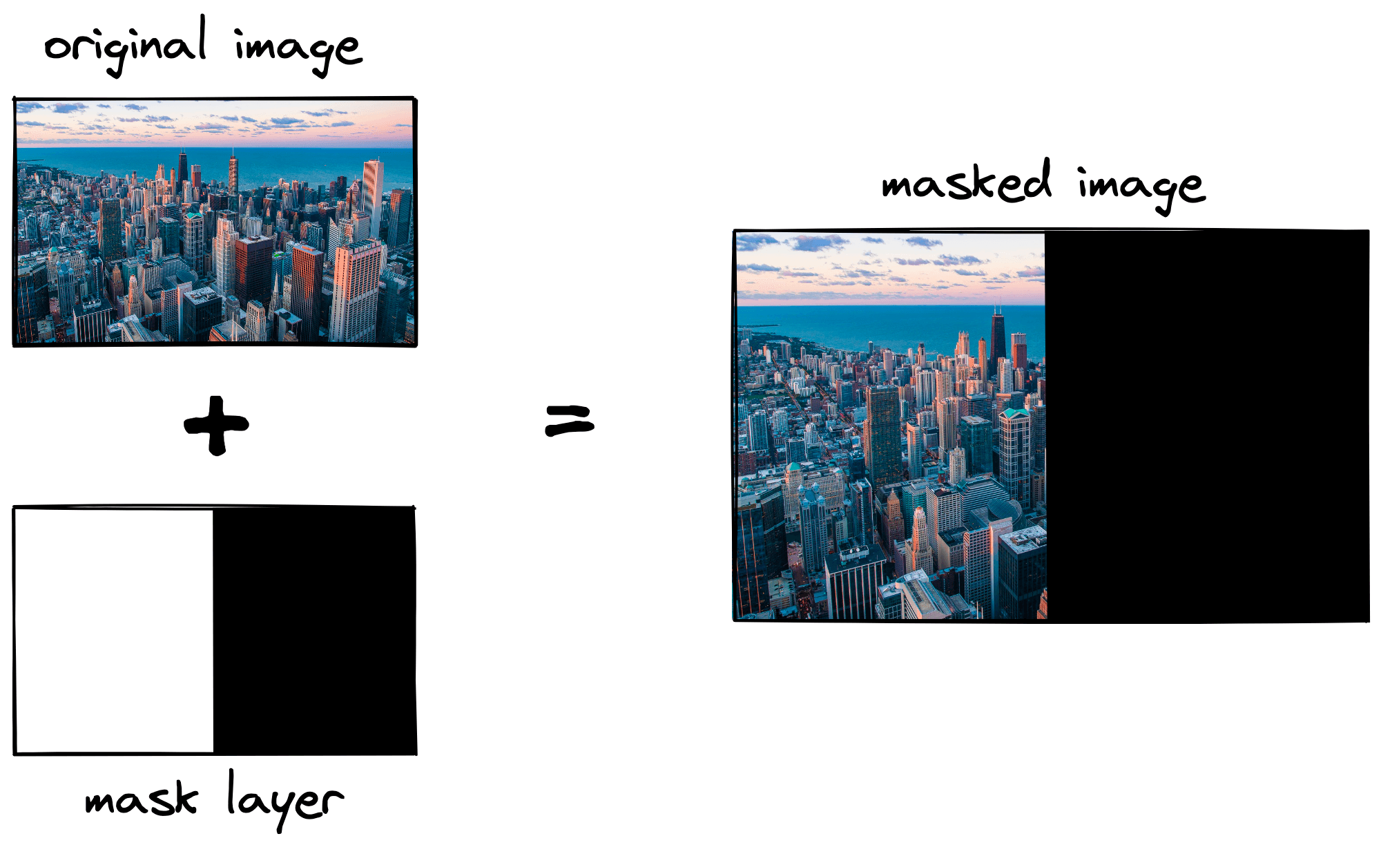
Example of how the masking layer works to “hide” part of an image.
binsis the number of buckets/histogram bars we place our values in. We can set this to 256 if we’d like to keep all of the original values.hist_rangeis the range of color values we expect. As we’re using RGB/BGR, we expect a min value of 0 and max value of 255, so we write[0, 256](the upper limit is exclusive).
After calculating these histogram values we can visualize them again using plot.
The calcHist function has effectively performed the same operation but with much less code. We now have our histograms; however, we’re not done yet.
Vectors and Similarity
We have a function for transforming our images into three vectors representing the three color channels. Before comparing our images we must concatenate these three vectors into a single vector. We will pack all of this into get_vector:
Using the default bins=32 this function will return a vector with 96 dimensions, where values [0, … 32] are red, [32, … 64] are green, and [64, … 96] are blue.
Once we have these vectors we can compare them using typical similarity/distance metrics such as Euclidean distance and cosine similarity. To calculate the cosine similarity we use the formula:

Which we write in Python with just:
def cosine(a, b):
    return np.dot(a, b) / (np.linalg.norm(a) * np.linalg.norm(b))
Using our cosine function we can calculate the similarity which varies from 0 (highly dissimilar) to 1 (identical). We can apply this alongside everything else we have done so far to create another search function that will return the top_k most similar images to a particular query image specified by its index idx in images.
We can add a few more components to this search function to output the images themselves rather than the image index positions; the code for this can be found here. Here are some of the results:
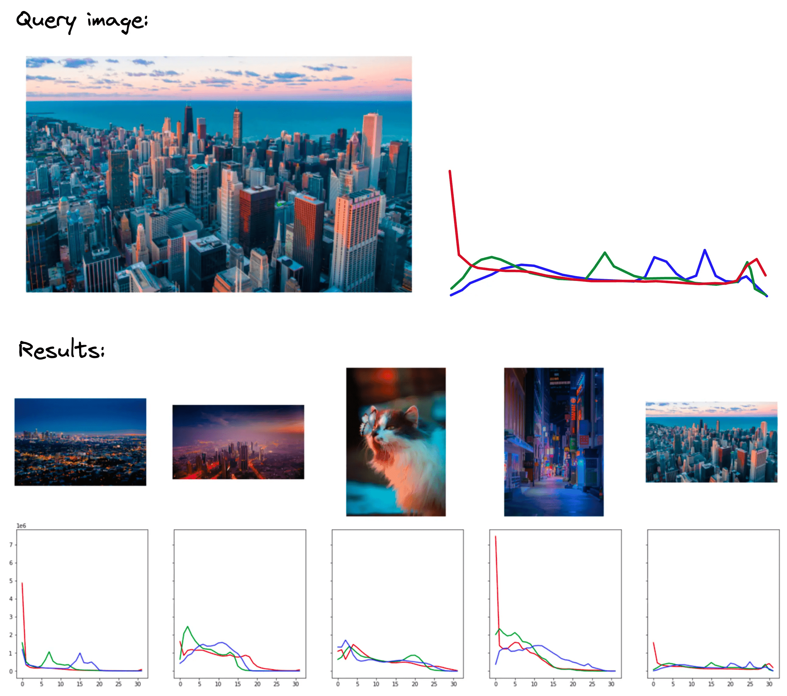
Color histogram retrieval with query image (top) and retrieved similar images (bottom).
Here, it is clear that the teal-orange color profile of the first query is definitely shared by the returned results. If we were looking for images with a similar aesthetic, I’d view this as a good result.
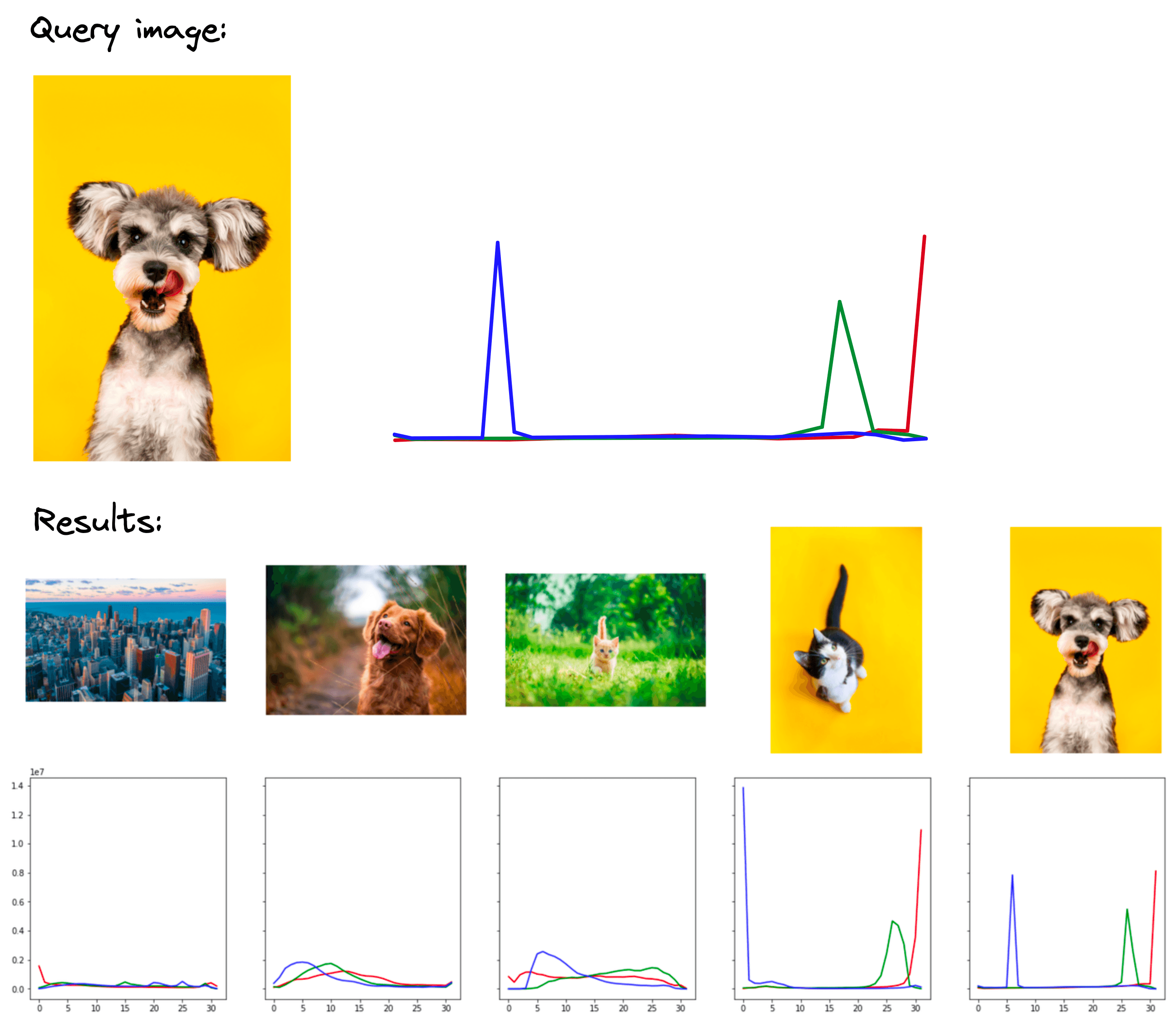
Color histogram retrieval with query image (top) and retrieved similar images (bottom).
The dog with orange background query returns a cat with orange background as the most similar result (excluding the same image). Again, in terms of color profiles and image aesthetics, the top result is good, and the histogram is also clearly similar.
These are some great results, and you can test the color histogram retrieval using the notebook here. However, this isn’t perfect, and these results can highlight some of the drawbacks of using color histograms.
Their key limitation is that they rely solely on image color profiles. That means the textures, edges, or actual meaning behind the content of images is not considered.
Further work on color histograms helped improve performance in some of these areas, such as comparing textures and edges, but these were still limited. Other deep learning methods greatly enhanced the performance of retrieving images based on semantic meaning, which is the focus of most modern technologies.
Despite these drawbacks, for a simple content-based image retrieval system, this approach provides several benefits:
- It is incredibly easy to implement; all we need to do is extract pixel color values and transform these into a vector to be compared with a simple metric like Euclidean distance or cosine similarity.
- The results are highly relevant for color-focused retrieval. If the meaningful content of an image is not important, this can be useful.
- Results are highly interpretable. There is no black box operation happening here; we know that every result is returned because it has a similar color profile.
With this in mind, embedding images using color histograms can produce great results for simple and interpretable image retrieval systems where aesthetics or color-profiles are important.
Resources
J. Smith, Integrated Spatial and Feature Image Systems: Retrieval, Analysis and Compression (2007)
Was this article helpful?