


Many of the most significant breakthroughs of AI and ML in the 2010s were theorized and described many decades ago. A few of the greatest ingredients to the AI gold-rush of the past decade are the perceptron (1958), backpropagation (1975), and (for NLP) recurrent neural networks (1986) [1, 2, 3].
How do seemingly obscure innovations from 1958, 1975, and 1986 become critical to a science and tech revolution in the 21st century?
They were not ‘rediscovered’; nothing was ever lost. Instead, the world at the time was not ready.
The many innovations that spurred AI forward over the last decade were ahead of their time, and their success required a few missing ingredients. The AI age was missing compute and data.
![Compute power (FLOPS) over time using a logarithmic scale. Source [4].](https://www.pinecone.io/_next/image/?url=https%3A%2F%2Fcdn.sanity.io%2Fimages%2Fvr8gru94%2Fproduction%2F986dccb4d91006e05bad11ae7e0c8078b885b08a-1920x1080.png&w=3840&q=75)
Compute power (FLOPS) over time using a logarithmic scale. Source [4].
Neural networks need many parameters to be effective. Look at some of the latest transformer models from the likes of OpenAI and Microsoft:
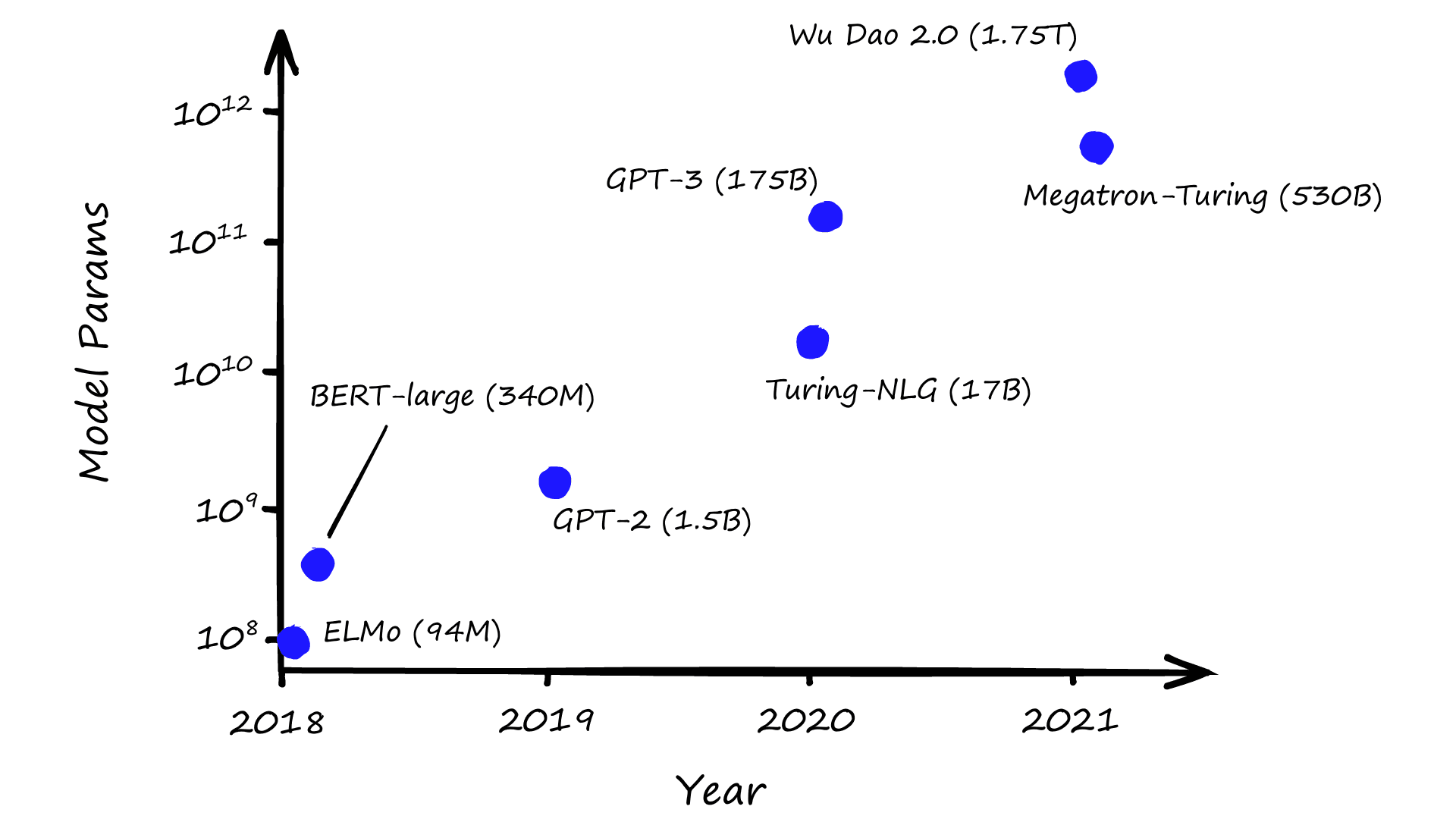
Model parameters over time, note the y-axis is using a log-scale.
Models have been getting bigger and bigger. With good reason, they perform better. Just how big they will get is anyone’s guess, but size matters, and,until very recently, there was not enough compute to train even the smallest models.
![Estimated data volume (worldwide) measured in zetabytes. Estimated values for 2021 are 79ZB compared to just 2ZB in 2010. Source [5]](https://www.pinecone.io/_next/image/?url=https%3A%2F%2Fcdn.sanity.io%2Fimages%2Fvr8gru94%2Fproduction%2Fa794b358e6d4b12cfc80e237a92b7eaa90584996-1920x1080.png&w=3840&q=75)
Estimated data volume (worldwide) measured in zetabytes. Estimated values for 2021 are 79ZB compared to just 2ZB in 2010. Source [5]
The second missing ingredient was data. ML models are data-hungry. They consume massive amounts of data to identify generalized patterns and apply those learned patterns to new data.
As models get bigger, so do datasets. And although we have seen an explosion of data in the past decade, it is often not accessible or in an ML-friendly format, especially in niche domains (such as climate-claim data) or low resource languages (Dhivehi, Navajo, etc).
Semantic search mostly requires the use of sentence transformers. Thanks to the improvements to computing power, finding the compute to train these models is not usually an issue. But, they’re big models and finding enough of the right data? That is a problem.
For many niche, low-resource domains, finding or annotating a substantial dataset manually is practically impossible.
We can try training without labeled data — but this only works for straight-forward semantic similarity tasks, and cannot produce as high-performing models as other supervised training methods (with labeled data).
Fortunately, we don’t need to label (or even find) this new data. Instead, we can automatically generate or label data using one or more data augmentation techniques.
In this article, we will introduce data augmentation and its application to the field of NLP. We will focus on the ‘in-domain’ flavor of a particular data-augmentation strategy named augmented SBERT (AugSBERT).
Data Augmentation
Data augmentation has been applied across the ML landscape and is not exclusive to NLP or sentence transformers. However, using data augmentation in NLP has proven to be a difficult task.
Augmentation is better developed within the field of computer vision (CV). It is relatively straightforward to apply many transformations that retain the ‘essence’ of an image while modifying pixel values. Images can be rotated, color graded, lightened/darkened, morphed, and more.
Language is more complex. It is more abstract and nuanced. Meaning is too easily corrupted by switching, replacing, deleting, or adding words. It is easy to end up with nonsensical gibberish.
The AugSBERT training strategy requires that we generate new sentence pairs that are:
- Sensible and on-topic
- Semantically and grammatically correct.
There are several ways we can build these new pairs, and we can mix several techniques. By far, the simplest is to randomly sample new sentence pairs.
Given just three sentence pairs where each sentence is unique we can generate six new pairs:
In[1]:
pairs = [
    ('I am sentence A', 'and this is sentence B'),
    ('there are three pairs', 'each pair includes an A and a B sentence'),
    ('random sampling creates more pairs', 'from these three, we create nine')
]
In[2]:
# mix all sentences
sampled = []
for a, _ in pairs:
    for _, b in pairs:
        print((a, b))
Out[2]:
('I am sentence A', 'and this is sentence B')
('I am sentence A', 'each pair includes an A and a B sentence')
('I am sentence A', 'from these three, we create nine')
('there are three pairs', 'and this is sentence B')
('there are three pairs', 'each pair includes an A and a B sentence')
('there are three pairs', 'from these three, we create nine')
('random sampling creates more pairs', 'and this is sentence B')
('random sampling creates more pairs', 'each pair includes an A and a B sentence')
('random sampling creates more pairs', 'from these three, we create nine')
As the number of original source or gold pairs increases, so does the number of generated silver pairs. Given 1,000 pairs we can generate 1,000,000 pairs. We will see later in the article that this approach is all we need to create a dataset large enough for training a sentence transformer.
(We refer to gold data as the high-quality original data, whereas silver is artificially generated, and therefore lower quality data.)
There are alternative techniques, and one of the more common options is the insertion or substitution of words. As mentioned, it is hard to do this without changing the meaning of a sentence, so we must approach insertion/substitution tactfully.
The nlpaug library covers many data augmentation techniques for NLP, including insertion and substitution using word embeddings using embedding methods like word2vec and fastText to ensure we insert/substitute relevant words:
![The original text (top) followed by a word2vec augmentation with insertion and substitution. Example from nlpaug [6].](https://www.pinecone.io/_next/image/?url=https%3A%2F%2Fcdn.sanity.io%2Fimages%2Fvr8gru94%2Fproduction%2F8614f03ffc690076917530ca9a9c691a0f4cccc1-1920x700.png&w=3840&q=75)
The original text (top) followed by a word2vec augmentation with insertion and substitution. Example from nlpaug [6].
We can even use context aware words embeddings with transformer models, including BERT, DistilBERT, RoBERTa, and XLNet.
![The original text (top) followed by a BERT augmentation with insertion and substitution. Example from nlpaug [6].](https://www.pinecone.io/_next/image/?url=https%3A%2F%2Fcdn.sanity.io%2Fimages%2Fvr8gru94%2Fproduction%2F00eaecc907e1b74969e5e805c3e51664d049d0b6-1920x740.png&w=3840&q=75)
The original text (top) followed by a BERT augmentation with insertion and substitution. Example from nlpaug [6].
nlpaug covers many other augmentation techniques, which are reviewed in-depth in the nlpaug GitHub repository [6]. However, we will be sticking with the random sampling strategy.
Augmented SBERT
Fine-tuning sentence transformer models require pairs of labeled data and lots of them.
The original SBERT was trained on 1M natural language inference (NLI) pairs, that is, 1M sentence pairs labeled as being highly related (entailment), contradictory, or neutral [7]. More recent models like flax-sentence-embeddings/all_datasets_v4_mpnet-base were trained on more than 1B sentence pairs [8].
When fine-tuning for a specific use case, it’s unlikely that we’ll find an existing and relevant dataset. That leaves us with two options:
- We manually annotate 100K+ sentence pairs
- We take 1-5K of existing (or manually annotated) sentence pairs and augment them with more data.
Under the assumption that you choose the latter option, how can we augment a dataset and generate realistic sentence pair labels? There are two steps: We use random sampling to create new pairs and then label them using a cross-encoder.
When comparing the semantic similarity of sentence pairs, we are not limited to sentence transformers (bi-encoders). We can use cross-encoder models too.
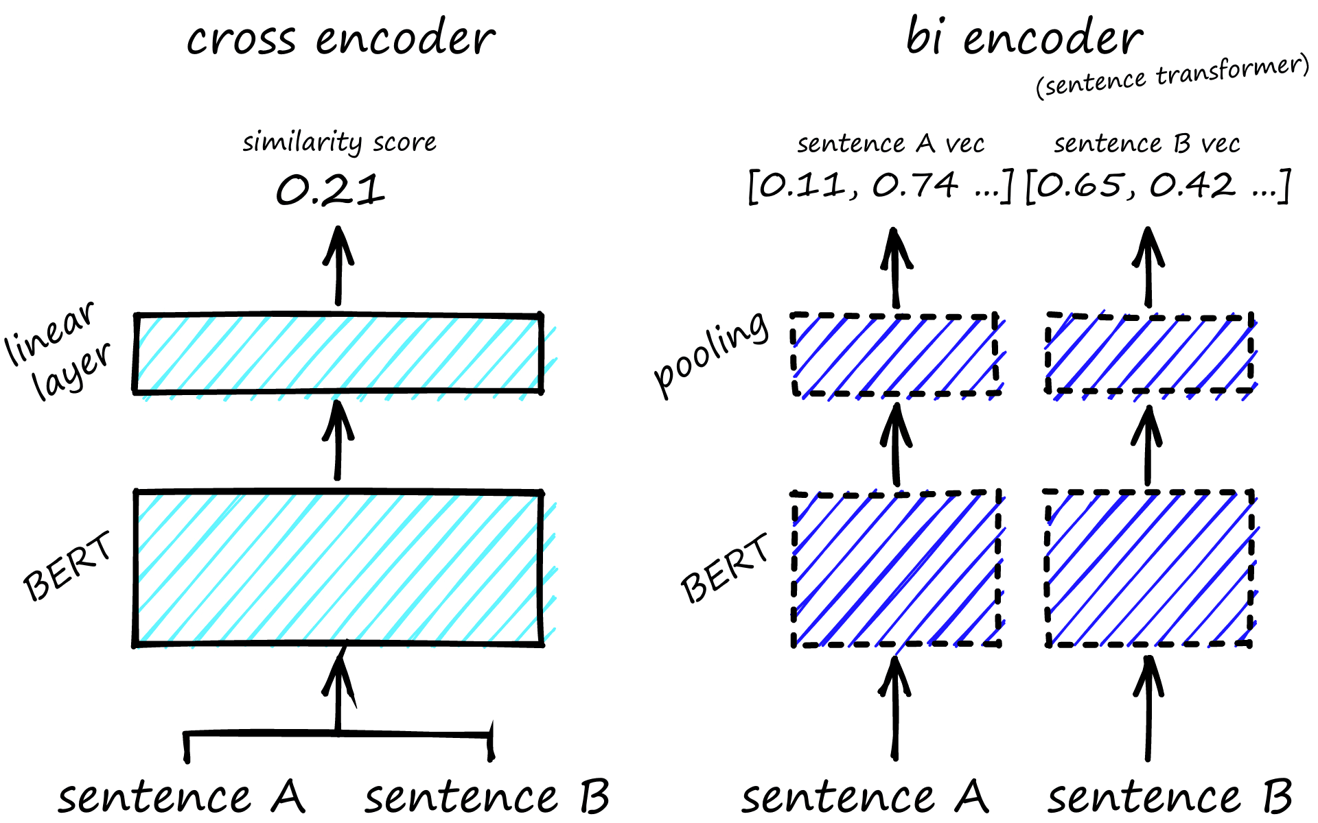
A cross-encoder (left) is a single BERT inference step that takes both sentences as a single input and outputs a similarity score. Bi-encoders (right) perform an inference step for each sentence and output sentence vectors.
Cross-encoders are more accurate than sentence transformers and require less data to train. However, this greater accuracy comes at a cost: Cross-encoders are much slower.
We must pass both sentence pairs to the cross-encoder, which outputs a similarity score.
The similarity score is often more accurate, but we had to perform a full cross-encoder (let’s assume we’re using BERT) inference step to get that single pairwise similarity.
If we need to search across a ‘small’ dataset containing 1M sentences? We need to perform 1M full-inference computations. That is slow.
Clustering with cross-encoders is an even more inefficient quadratic complexity [7]. For clustering, we must compare every single pair. For all but the tiniest datasets, this is too slow to be usable in most use-cases.
On the other hand, sentence transformers require us to encode each sentence to produce a sentence vector. We will need to run 1M full inference computations on our first run to create these vectors, but once we have them, we store them in a database/index for quicker lookups.
Given a new sentence, performing a search across that same small dataset of 1M sentence vectors means we encode the new sentence (one inference computation) and then calculate the Euclidean/cosine similarity between that one vector and the 1M already indexed sentence vectors.
1M cosine similarity computations are faster than 1M full BERT inference computations. Additionally, with sentence vectors, we can use approximate nearest neighbors search (ANNS) to speed up the process even further.
A BERT cross-encoder can take 65 hours to cluster 10K sentences. The equivalent process with SBERT takes five seconds [7].
When to Use AugSBERT
We will assume one of two scenarios:
- We have found an existing labeled dataset, but it is tiny,maybe just 1-5K pairs or
- We have an unlabeled dataset, but it is within reason to manually label (annotate) at least 1-5K pairs.
We have a small but annotated dataset. We could try fine-tuning a sentence transformer, but it is unlikely to perform well. Instead, we can turn to augmentation to enhance our dataset and improve the potential sentence transformer performance.
There are now the two steps we mentioned earlier to create this data. First, we generate more pairs, for which we will use random sampling. Second, we label that new data with a cross-encoder fine-tuned on the original (smaller) dataset.
Random sampling is used to enlarge the number of sentence pairs in our dataset. After producing this larger dataset, we use the cross-encoder to label the new pairs.
Because cross-encoders require fewer data and produce high-accuracy similarity scores, they’re great for annotating our unlabeled data. With more labeled data, we can fine-tune better-performing sentence transformers.
The Augmented SBERT (AugSBERT) fine-tuning strategy is ideal for training with tiny datasets. Evaluation of the strategy showed improvements of up to 6% for in-domain tasks and up to 37% for domain adaption tasks [9].
The training process always begins with a gold dataset. Gold is our already labeled and (hopefully) high-quality data. If you can’t get gold, the next best thing is silver. Likewise, the next best ‘augmented data’ is named the silver dataset.
We feed the gold and unlabeled data into a BERT cross-encoder, producing our silver data. The SBERT bi-encoder is fine-tuned with this gold and silver data.
At a high level, this is how in-domain AugSBERT training works. Let’s flesh out the details and work through an example.
In-Domain Walkthrough
To implement the in-domain AugSBERT training strategy, we need to have a small amount of labeled data within the same domain that we’d like to fine-tune our sentence transformer. We can then use this to generate more in-domain data.
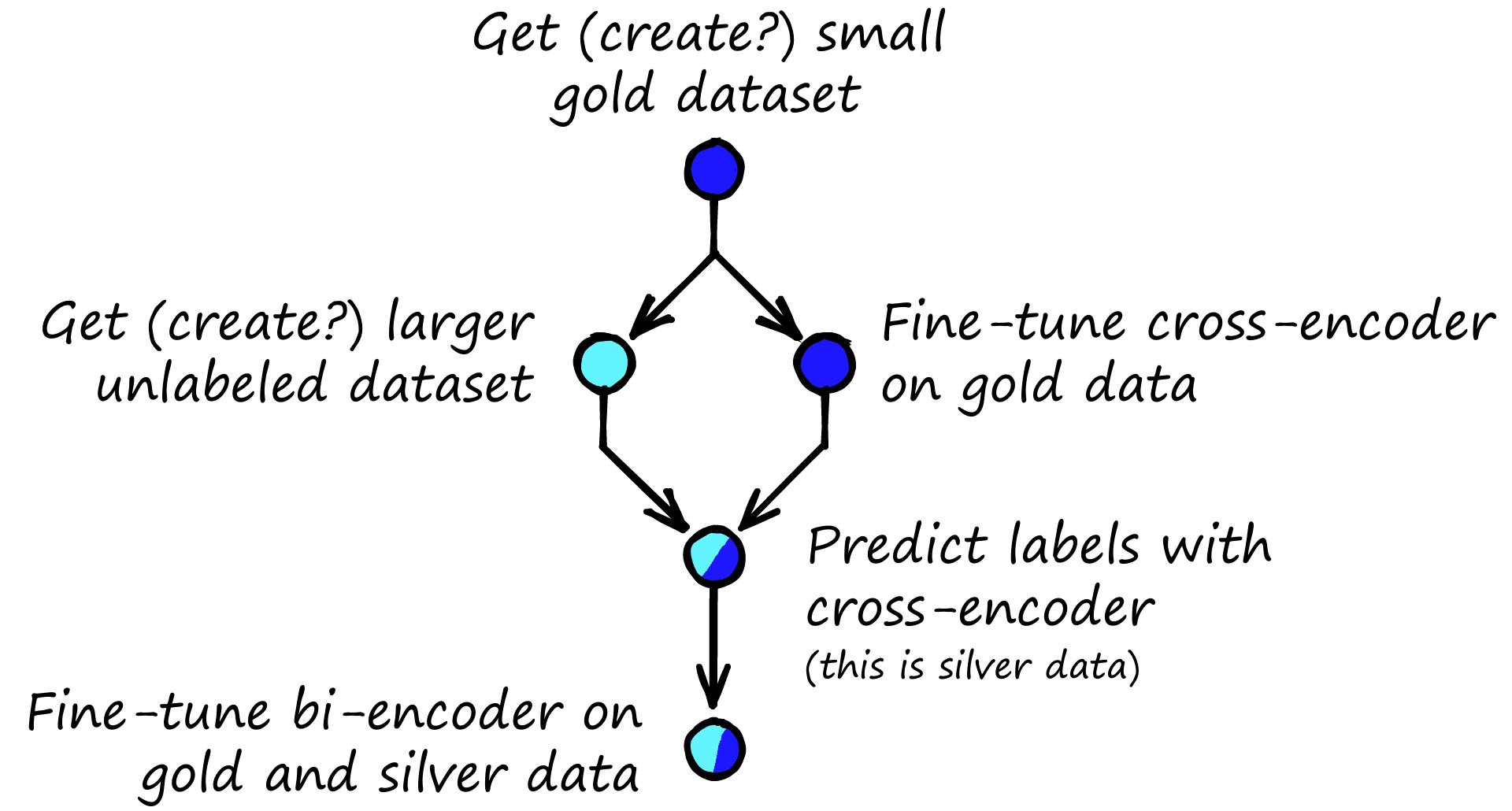
Step-by-step process for fine-tuning a sentence transformer (bi-encoder) with the AugSBERT in-domain strategy.
We can use this gold data to fine-tune the sentence transformer. The problem is that we do not have enough data. So, we must generate more data, or if there is already unlabeled data available, we can label that directly.
We will use the Semantic Textual Similarity benchmark (STSb) dataset. It is available via the 🤗 Datasets library. It contains just 5,749 pairs, very little for fine-tuning a sentence transformer model.
In[1]:
import datasets

stsb = datasets.load_dataset('glue', 'stsb', split='train')
stsb_dev = datasets.load_dataset('glue', 'stsb', split='validation')
stsb
Out[1]:
Dataset({
    features: ['sentence1', 'sentence2', 'label', 'idx'],
    num_rows: 5749
})
After normalizing the label feature to between 0 -> 1, each row in our dataset will look something like this:
{
'sentence1': 'A plane is taking off.',
'sentence2': 'An air plane is taking off.',
'label': 1.0, # this value will range from 0.0 -> 1.0
'idx': 0
}
We have 5,749 pairs in the train set and 1,500 pairs in the validation (or dev) set. Fine-tuning with this core gold dataset produces a model that scores 0.506 using Spearman’s correlation with those dev set labels, where 0.0 means no correlation and 1.0 is an exact match or perfect correlation.
We can improve this score using an in-domain AugSBERT training strategy, which begins by training a cross-encoder using this small gold dataset.
Fine-Tune Cross-Encoder
Before training, we must reformat our training to a list of InputExamples and use them to initialize a DataLoader.
In[3]:
from sentence_transformers import InputExample
from torch.utils.data import DataLoader

train_data = []
for row in stsb:
    train_data.append(
        InputExample(
            texts=[row['sentence1'], row['sentence2']],
            label=int(float(row['label']))
        )
    )

batch_size = 16
# load our training data (first 95%) into a dataloader
loader = DataLoader(
    train_data, shuffle=True, batch_size=batch_size
)
We then initialize and fine-tune our cross encoder.
In[5]:
from sentence_transformers.cross_encoder import CrossEncoder

cross_encoder = CrossEncoder('bert-base-uncased', num_labels=1)
In[6]:
num_epochs = 1
warmup = int(len(loader) * num_epochs * 0.4)

cross_encoder.fit(
    train_dataloader=loader,
    epochs=num_epochs,
    warmup_steps=warmup,
    output_path='bert-stsb-cross-encoder'
)
Out[6]:
Iteration: 100%|██████████| 360/360 [00:21<00:00, 17.09it/s]
Epoch: 100%|██████████| 1/1 [00:22<00:00, 22.51s/it]
The number of warmup steps is 40% of the total training steps. It is high but helps prevent overfitting. The same could likely be achieved using a lower learning rate (the default is 2e-5).
Evaluation of the cross-encoder model on the dev set returns a correlation score of 0.578.
Create Unlabeled Data
The cross-encoder is one half of the recipe for building a silver dataset, and the other half are the unlabeled sentence pairs. There are different strategies for generating this data, but one of the simplest and most effective is to randomly sample pairs from the gold data, creating new sentence pairs.
For this, we can transform the pairs from dataset objects to Pandas DataFrames, as these provide easy-to-use sampling methods.
In[3]:
import pandas as pd

gold = datasets.load_dataset('glue', 'stsb', split='train')

gold = pd.DataFrame({
    'sentence1': gold['sentence1'],
    'sentence2': gold['sentence2']
})
We can then initialize a new pairs dataframe, loop through each unique sentence from the sentence1 column and find new pairs from the sentence2 column.
In[3]:
from tqdm.auto import tqdm


pairs = pd.DataFrame()
# loop through each unique sentence in 'sentence1'
for sentence1 in tqdm(list(set(gold['sentence1']))):
    # get a sample of 5 rows that do not contain the current 'sentence1'
    sampled = gold[gold['sentence1'] != sentence1].sample(5)
    # get the 5 sentence2 sentences
    sampled = sampled['sentence2'].tolist()
    for sentence2 in sampled:
        # append all of these new pairs to the new 'pairs' dataframe
        pairs = pairs.append({
            'sentence1': sentence1,
            'sentence2': sentence2
        }, ignore_index=True)
Out[3]:
100%|██████████| 5436/5436 [00:39<00:00, 138.94it/s]
Finally, we should drop any duplicates from the new pairs data.
In[5]:
pairs = pairs.drop_duplicates()
len(pairs)
With that, we have 27,180 unlabeled sentence pairs; the second half needed to build a fully labeled silver dataset.
Labeling the Silver Dataset
We generate label predictions for the unlabeled data using the cross-encoder that we trained. It is this cross-encoder-labeled data that we refer to as the silver dataset.
![In-domain training strategy with AugSBERT, source [9]. We feed unlabeled pairs into the fine-tuned cross-encoder to create the silver dataset.](https://www.pinecone.io/_next/image/?url=https%3A%2F%2Fcdn.sanity.io%2Fimages%2Fvr8gru94%2Fproduction%2F19b573408ab4196937afbffdc23b507cade880ae-1920x1200.png&w=3840&q=75)
In-domain training strategy with AugSBERT, source [9]. We feed unlabeled pairs into the fine-tuned cross-encoder to create the silver dataset.
Earlier we saved the cross-encoder to file in the local bert-stsb-cross-encoder directory. To load it from file we use:
In[6]:
from sentence_transformers.cross_encoder import CrossEncoder
cross_encoder = CrossEncoder('bert-stsb-cross-encoder')
Then we predict new labels for our unlabeled data.
In[7]:
# zip pairs together in format for the cross-encoder
silver = list(zip(pairs['sentence1'], pairs['sentence2']))
# predict labels for the unlabeled silver data
scores = cross_encoder.predict(silver)

# add the predicted scores to the pairs dataframe
pairs['label'] = scores.tolist()
pairs.head()
Out[7]:
                                           sentence1  \
0  Stanford (51-17) and Rice (57-12) will play fo...
1  Stanford (51-17) and Rice (57-12) will play fo...
2  Stanford (51-17) and Rice (57-12) will play fo...
3  Stanford (51-17) and Rice (57-12) will play fo...
4  Stanford (51-17) and Rice (57-12) will play fo...

                                           sentence2     label
0                                  Kids are dancing.  0.014961
1  If so, alot of inventors, writers should take ...  0.014872
2  Time of the Season by the Zombies We are all v...  0.014914
3        St. Bernard dog running in the snowy field.  0.013343
4                       The dog is running on grass.  0.014792
We now have both gold and silver datasets to fine-tune the sentence transformer, a total of 5_749 + 27_180 == 32_929 pairs. Now, we can fine-tune the sentence transformer.
Fine-Tune Sentence Transformer
Before training, we need to merge the silver and gold datasets; with both as Pandas DataFrame objects, we use append. As before, we also transform our data into a list of InputExample objects and use them to initialize a DataLoader.
all_data = gold.append(pairs, ignore_index=True)

# format into input examples
train = []
for _, row in all_data.iterrows():
    train.append(
        InputExample(
            texts=[row['sentence1'], row['sentence2']],
            label=float(row['label'])
        )
    )

# initialize dataloader
loader = DataLoader(
    train, shuffle=True, batch_size=batch_size
)
Our data is ready for training, so we initialize our model. The model consists of a core transformer model, in this case, bert-base-uncased from 🤗 Transformers. Following this, we have a pooling layer, which transforms the 512 token-level vectors into single sentence vectors. We will use the mean pooling method.
from sentence_transformers import models, SentenceTransformer

# initialize model
bert = models.Transformer('bert-base-uncased')
pooler = models.Pooling(
    bert.get_word_embedding_dimension(),
    pooling_mode_mean_tokens=True
)
model = SentenceTransformer(modules=[bert, pooler])
We must define a loss function to optimize on. We will use a cosine similarity loss function as we have similarity scores in the dataset.
from sentence_transformers import losses

loss = losses.CosineSimilarityLoss(model=model)
Then we begin training. We use the default learning rate and warmup for the first 15% of steps.
# and training
epochs = 1
# warmup for first 15% of training steps
warmup_steps = int(len(loader) * epochs * 0.15)

model.fit(
    train_objectives=[(loader, loss)],
    epochs=epochs,
    warmup_steps=warmup_steps,
    output_path='bert-stsb-aug'
)
With that, we have fine-tuned our STSb sentence transformer using the in-domain AugSBERT training strategy. To evaluate the model, we run a small evaluation script, which returns the correlation score with pairs from the STSb dev set.
| Model | Score | Note |
|---|---|---|
| bert-stsb-aug | 0.691 | BERT-base uncased model fine-tuned on the gold and silver STSb data. |
| bert-stsb-gold | 0.506 | BERT-base uncased model fine-tuned on the gold STSb data only (no dataset augmentation). |
| bert-stsb-cross-encoder | 0.692 | BERT-base uncased cross-encoder model fine-tuned on the gold STSb data. Used to create the silver data. |
We return some incredible results for the sentence transformer fine-tuned using the AugSBERT strategy, returning almost 19% better performance than the model fine-tuned on the gold dataset only.
The paper introducing AugSBERT demonstrated performance increases of up to six points for in-domain tasks. So, it’s worth assuming that the 19-point improvement here is very high and an atypical improvement. However, it shows just how good an AugSBERT training strategy can be.
That’s it for fine-tuning using the in-domain Augmented SBERT strategy. The renaissance of ML we are currently witnessing may have been ignited by 50-70s research and enabled through massive advances in compute availability, but without the right data, we’re stuck.
It is with new techniques like AugSBERT that we are finally able to traverse the last mile and bridge those gaps in data.
We’ve introduced the idea of data augmentation in the field of NLP and how we can use insertion/substitution or simple random sampling techniques to generate new sentence pairs (e.g., the silver dataset).
We learned about cross encoders, bi-encoders, and how we can label our silver data using cross encoders.
Finally, we fine-tuned our bi-encoder or ‘sentence transformer’ using gold and silver datasets and evaluated its performance against another bi-encoder trained without the AugSBERT strategy.
With this strategy, we can apply semantic similarity models to niche domains that have not been caught in the swell of data from the past decade.Demonstrating that AugSBERT can be a convenient approach to enhancing model performance in these domains.
References
[1] F. Rosenblatt, The Perceptron: A Probabilistic Model For Information Storage and Organization in the Brain (1958), PsycINFO
[2] P. Werbos, Beyond Regression: New Tools For Prediction and Analysis in the Behavioral Sciences (1974), Harvard University
[3] D. Rumelhard, et al., Learning Representations by Back-Propagating Errors (1986), Nature
[4] Top500 Supercomputer Leaderboards
[5] A. Holst, Volume of data/information created, copied, and consumed worldwide from 2010 to 2025 (2021), Statistica
[6] E. Ma, nlpaug, GitHub
[7] N. Reimers, I. Gurevych, Sentence-BERT: Sentence Embeddings using Siamese BERT-Networks (2019), EMNLP 2019
[8] Model Card for all_datasets_v4_mpnet-base, HuggingFace Models
[9] N. Thakur, et al., Augmented SBERT: Data Augmentation Method for Improving Bi-Encoders for Pairwise Sentence Scoring Tasks (2021), NAACL
Was this article helpful?