











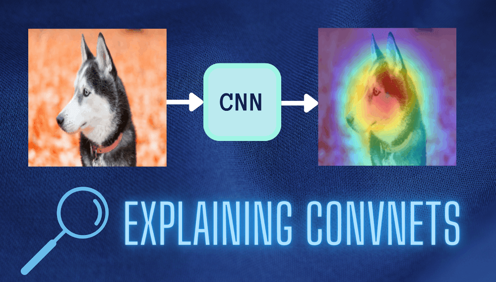
Have you ever used deep learning to solve computer vision tasks? If so, you probably trained a convolutional neural network (ConvNet or CNN) for tasks such as image classification and visual question answering.
In practice, ConvNets are often viewed as black boxes that take in a dataset and give a task-specific output: predictions in image classification, captions in image captioning, and more. For example, in image classification, you’ll optimize the model for prediction accuracy.
But how do you know which parts of the image the network was looking at when it made a prediction? And how do you go from black box to interpretable models?
Adding a layer of explainability to ConvNets can be helpful in applications such as medical imaging for disease prognosis. For example, consider a classification model trained on medical images, namely, brain scans and X-rays, to predict the presence or absence of a medical condition. Ensuring that the model is using the relevant parts of the images for its predictions makes it more trustworthy than a black box model with a high prediction accuracy.
Class activation maps can help explain the predictions of a ConvNet. Class activation maps, commonly called CAMs, are class-discriminative saliency maps. While saliency maps give information on the most important parts of an image for a particular class, class-discriminative saliency maps help distinguish between classes.
In this tutorial, you’ll learn how class activation maps (CAM) and their generalizations, Grad-CAM and Grad-CAM++, can be used to explain a ConvNet. You’ll then learn how to generate class activation maps in PyTorch.
Let’s begin!
In general, a ConvNet consists of a series of convolutional layers, each consisting of a set of filters, followed by fully connected layers.
Activation maps indicate the salient regions of an image for a particular prediction. Class activation map (CAM) uses a global average pooling (GAP) layer after the last convolutional layer. Let’s understand how this works.
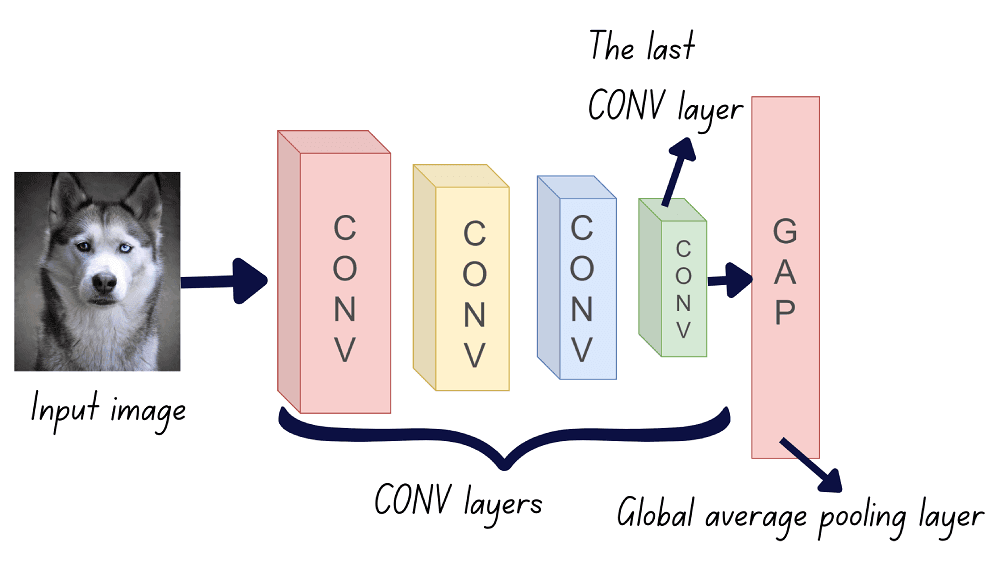
GAP Layer After the Last CONV Layer (Image by the author)
If there are n filters in the last convolutional layer, then there are n feature maps. The activation map for a particular output class is the weighted combination of all the n feature maps.
So how do we learn these weights?
Step 1: Apply global average pooling to each of the feature maps.
The average value of all pixels in a feature map is its global average. Here’s an example of how global average pooling works. The qualifier global means that the average is computed over all pixel locations in the feature map.
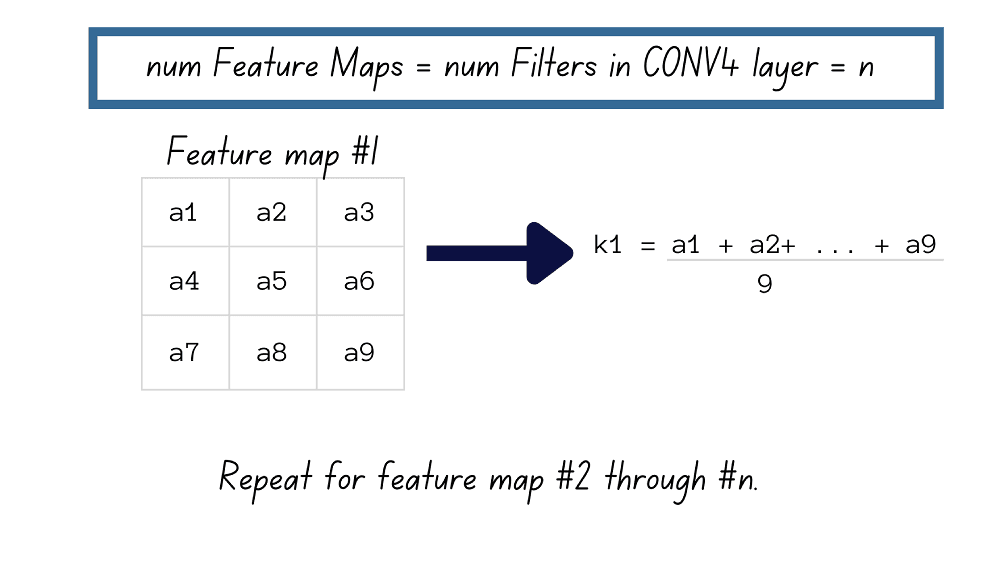
How GAP Works - An Example (Image by the author)
After computing the global average for each of the feature maps, we’ll have n scalars, . Let’s call them GAP outputs.
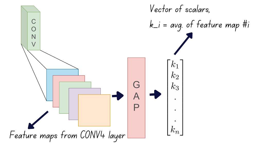
From Feature Maps to Scalars through GAP (Image by the author)
Step 2: The next step is to learn a linear model from these GAP outputs onto the class labels. For each of the N output classes, we should learn a model with weights . Therefore, we’ll have to learn N linear models in all.
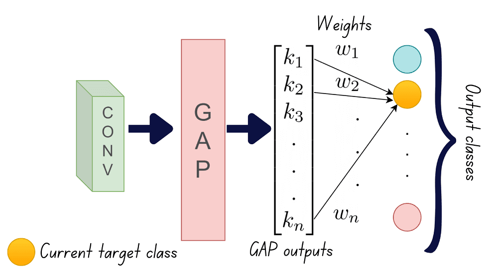
Linear Models from GAP Output onto the Class Labels (Image by the author)
Step 3: Once we’ve obtained the n weights for each of the N classes, we can weight the feature maps to generate the class activation maps. Therefore, different weighted combinations of the same set of feature maps give the class activation maps for the different classes.

Class Activation Maps as Weighted Combinations of Feature Maps (Image by the author)
Mathematically, the class score for an output class c in the CAM model is given by:
Even though we need to train N linear models to learn the weights, CAM does not require a backward pass through the network again. A backward pass through the layers of the network is more expensive than learning a linear mapping.
CAM uses the inherent localization capability of the convolutional layers, so the activation maps can be generated without any positional supervision on the location of the target in the image.
Using class activation maps involves the overhead of learning N linear models to learn the weights for each of the N classes. Training a ConvNet is a computationally intensive task in itself. This overhead can be a limiting factor when both n, the number of filters in the last convolutional layer, and N, the number of output classes, are especially large.
The introduction of the global average pooling (GAP) layer after the last convolutional layer imposes a restriction on the ConvNet architecture. Though CAM is helpful in explaining the predictions in an image classification task, it cannot be used for computer vision tasks such as visual question answering (VQA). As explained, the GAP layer outputs are scalars that are global averages of the preceding convolutional layer’s feature maps. There is no known performance degradation for image classification. However, this requirement for the GAP layer after the convolutional layers may be too restrictive for tasks like VQA.
As mentioned, the key limitation of CAM is the overhead of learning the weights for linear mapping. Gradient-weighted class activation map (Grad-CAM) is a generalization to CAM that overcomes this limitation.
Let’s start by making a simple substitution in the equation for output class score in CAM.
Next, let’s compute the derivative of the output class score with respect to the pixels in the feature map.
Summing the above quantities over all the pixels in the feature map, we have the following:
As seen in the above equation, the weights evaluate to the gradient of the output score with respect to the kth feature map. This means there’s no need to retrain N linear models to learn the weights!
We’ve summed over all pixel locations (i,j). Adding the normalization factor 1/Z back in, we get:
In essence, Grad-CAM uses the global average of the gradients flowing into the feature maps of the last convolutional layer.
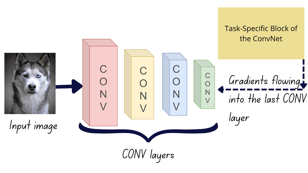
How Grad-CAM Works (Image by the author)
To retain only the positive correlations in the final activation map, we apply the ReLU function on the weighted combination of feature maps.
ReLU function: f(x) = ReLU(x) = x if x >= 0 and 0 otherwise. The ReLU function filters all the negative inputs and passes the positive inputs as they are.
Given that the gradients of the output with respect to the feature maps identify salient patches in the image, what do negative gradients signify?
Using negative gradients in the weights will give those patches in the image that adversarially affect a particular prediction. For example, in an image containing a cat and a dog, if the target class is cat, then the pixel patch corresponding to the dog class affects prediction.
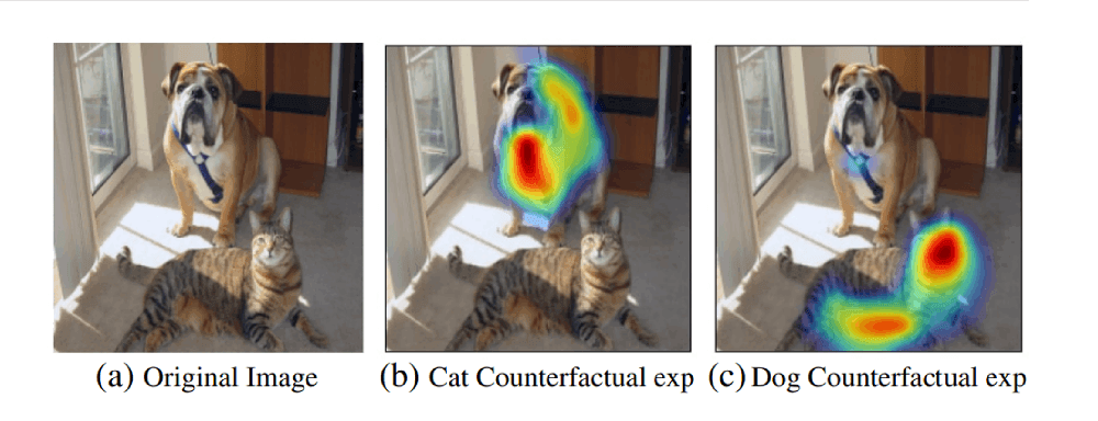
Grad-CAM Counterfactual Explanations
Therefore, by identifying and removing these patches from the images, we can suppress the adversarial effect on prediction. As a result, the confidence of prediction increases.
Even though Grad-CAM provides activation maps with good target localization, it fails to capture certain minute details. Pixel-space gradient visualization techniques, which were used in earlier approaches to explainability, can provide more granular information on which pixels have the most influence.
To obtain a detailed activation map, especially to understand misclassifications among similar classes, we can use guided backpropagation in conjunction with Grad-CAM. This approach is called guided Grad-CAM.
The concept of guided backpropagation was introduced in [2]. Given a feedforward neural network, the influence of an input x_j on a hidden layer unit h_i is given by the gradient of h_i with respect to x_j. This gradient can be interpreted as follows:
So to understand the fine-grained details, we only backpropagate along the path with positive gradients. Since this approach uses information from higher layers during the backprop, it’s called guided backpropagation.
N models to explain the ConvNet’s prediction.When there are multiple occurrences of the target class within a single image, the spatial footprint of each of the occurrences is substantially lower. Grad-CAM fails to provide convincing explanations under such “low spatial footprint” conditions.
Grad-CAM++ provides better localization when the targets have a low spatial footprint in the images.
Let’s start by reviewing the equation for the Grad-CAM weights.
From the above equation, we see that Grad-CAM scales all pixel gradients by the same factor 1/Z. This means that each pixel gradient has the same significance in generating the final activation map. However, in images where the target has a low spatial footprint, the pixel gradients that actually help the prediction should have greater significance.
To achieve this, Grad-CAM++ proposes the following:
Mathematically, this can be expressed as:
Let’s parse what means.
Applying the ReLU function on the gradients ensures that only the gradients that have a positive contribution to the class prediction are retained.
Working out the math like we did for Grad-CAM, the values of can be given by the following closed-form expression:
Unlike Grad-CAM weights that use first-order gradients, Grad-CAM++ weights use higher order gradients (second and third-order gradients).
The output activation map is given by:
Now that you’ve learned how class activation maps and the variants, Grad-CAM and Grad-CAM++, work, let’s proceed to generate class activation maps for images.
The PyTorch Library for CAM Methods by Jacob Gildenblat and contributors on GitHub has ready-to-use PyTorch implementations of Grad-CAM, Grad-CAM++, EigenCAM, and much more. This library grad-cam is available as a PyPI package that you can install using pip.
📥 Download the Colab notebook and follow along.
You can customize this generic CAM example depending on the computer vision task to which you’d like to add explainability. Let’s start by importing the necessary modules.
from torchvision import models
import numpy as np
import cv2
import PIL
Next, we import the necessary classes from the grad_cam library.
from pytorch_grad_cam import GradCAM,GradCAMPlusPlus
from pytorch_grad_cam.utils.model_targets import ClassifierOutputTarget
from pytorch_grad_cam.utils.image import show_cam_on_image,preprocess_image
In this example, we’ll use the pre-trained ResNet50 model from the PyTorch Torchvision library that contains datasets and pre-trained models. We then define the target class, the layer after which we’d like to generate the activation map. In this example, we’ve used the following ImageNet classes: Goldfish, Siberian Husky, and Mushroom.
# use the pretrained ResNet50 model
model = models.resnet50(pretrained=True)
model.eval()

# fix target class label (of the Imagenet class of interest!)
# 1: goldfish, 250: Siberian Husky, 947: mushroom

targets = [ClassifierOutputTarget(<target-class-number>)]

# fix the target layer (after which we'd like to generate the CAM)
target_layers = [model.layer4]
We can instantiate the model, preprocess the image, generate and display the class activation map.
# instantiate the model
cam = GradCAM(model=model, target_layers=target_layers) # use GradCamPlusPlus class

# Preprocess input image, get the input image tensor
img = np.array(PIL.Image.open('<image-file-path>'))
img = cv2.resize(img, (300,300))
img = np.float32(img) / 255
input_tensor = preprocess_image(img)

# generate CAM
grayscale_cams = cam(input_tensor=input_tensor, targets=targets)
cam_image = show_cam_on_image(img, grayscale_cams[0, :], use_rgb=True)

cam = np.uint8(255*grayscale_cams[0, :])
cam = cv2.merge([cam, cam, cam])

# display the original image & the associated CAM
images = np.hstack((np.uint8(255*img), cam_image))
PIL.Image.fromarray(images)
We can interpret the class activation map as a heatmap in which the regions in red are the most salient for a particular prediction, and the regions in blue are the least salient.
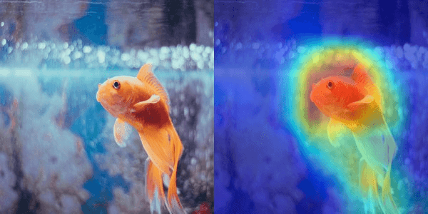
Activation Map for Class Goldfish (ImageNet Class #1)
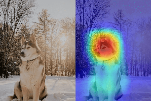
Activation Map for Class Siberian Husky (ImageNet Class #250)
So far, the targets were present only once in the entire image. Now, consider the following image with many small mushrooms, each having a very small spatial footprint.
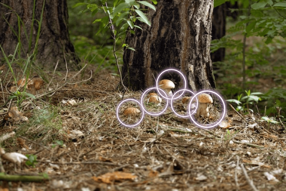
In this case, the activation map generated using GradCAM++ better identifies all instances of mushroom than the one from GradCAM.
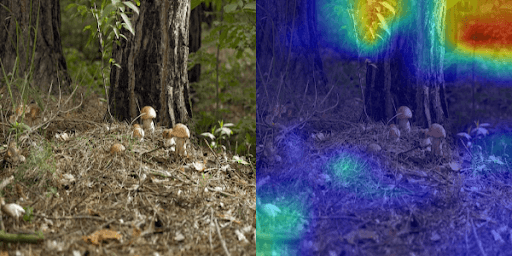
Grad-CAM Output for Multiple Occurrences of Class Mushroom (ImageNet Class #947)
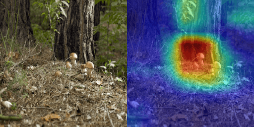
Grad-CAM++ Output for Multiple Occurrences of Class Mushroom (ImageNet Class #947)
As a next step, you can try generating activation maps for any class or other vision task of your choice.
I hope you enjoyed this tutorial on explaining ConvNets with activation maps. Here’s a summary of what you’ve learned.
If you’d like to delve deeper, consider checking out the resources below. Happy learning!
[1] Bolei Zhou et al., Learning Deep Features for Discriminative Localization, 2015
[2] Springenberg and Dosovitskiy et al., Striving for Simplicity: The All Convolutional Net, ICLR 2015
[3] R Selvaraju et al., Grad-CAM: Visual Explanations from Deep Networks via Gradient-Based Localizations, ICCV 2017
[4] A Chattopadhyay et al., Grad-CAM++: Improved Visual Explanations for Deep Convolutional Networks, WACV 2018
[5] B Zhou et al., Object Detectors Emerge in Deep Scene CNNs, ICLR 2015
[6] Jacob Gildenblat and contributors, PyTorch Library for CAM Methods, GitHub, 2021
此内容由惯性聚合(RSS阅读器)自动聚合整理,仅供阅读参考。 原文来自 — 版权归原作者所有。