


Our article introducing sentence embeddings and transformers explained that these models can be used across a range of applications, such as semantic textual similarity (STS), semantic clustering, or information retrieval (IR) using concepts rather than words.
This article dives deeper into the training process of the first sentence transformer, sentence-BERT, or more commonly known as SBERT. We will explore the Natural Language Inference (NLI) training approach of softmax loss to fine-tune models for producing sentence embeddings.
Be aware that softmax loss is no longer the preferred approach to training sentence transformers and has been superseded by other methods such as MSE margin and multiple negatives ranking loss. But we’re covering this training method as an important milestone in the development of ever improving sentence embeddings.
This article also covers two approaches to fine-tuning. The first shows how NLI training with softmax loss works. The second uses the excellent training utilities provided by the sentence-transformers library — it’s more abstracted, making building good sentence transformer models much easier.
NLI Training
There are several ways of training sentence transformers. One of the most popular (and the approach we will cover) is using Natural Language Inference (NLI) datasets.
NLI focus on identifying sentence pairs that infer or do not infer one another. We will use two of these datasets; the Stanford Natural Language Inference (SNLI) and Multi-Genre NLI (MNLI) corpora.
Merging these two corpora gives us 943K sentence pairs (550K from SNLI, 393K from MNLI). All pairs include a premise and a hypothesis, and each pair is assigned a label:
- 0 — entailment, e.g. the
premisesuggests thehypothesis. - 1 — neutral, the
premiseandhypothesiscould both be true, but they are not necessarily related. - 2 — contradiction, the
premiseandhypothesiscontradict each other.
When training the model, we will be feeding sentence A (the premise) into BERT, followed by sentence B (the hypothesis) on the next step.
From there, the models are optimized using softmax loss using the label field. We will explain this in more depth soon.
For now, let’s download and merge the two datasets. We will use the datasets library from Hugging Face, which can be downloaded using !pip install datasets. To download and merge, we write:
In[1]:
import datasets

snli = datasets.load_dataset('snli', split='train')

snli
Out[1]:
Dataset({
    features: ['premise', 'hypothesis', 'label'],
    num_rows: 550152
})
Out[2]:
{'premise': 'A person on a horse jumps over a broken down airplane.', 'hypothesis': 'A person is training his horse for a competition.', 'label': 1}
In[3]:
m_nli = datasets.load_dataset('glue', 'mnli', split='train')

m_nli
Out[3]:
Dataset({
    features: ['premise', 'hypothesis', 'label', 'idx'],
    num_rows: 392702
})
In[4]:
m_nli = m_nli.remove_columns(['idx'])
snli = snli.cast(m_nli.features)
dataset = datasets.concatenate_datasets([snli, m_nli])
Out[4]:
Dataset({
    features: ['premise', 'hypothesis', 'label'],
    num_rows: 942854
})
Both datasets contain -1 values in the label feature where no confident class could be assigned. We remove them using the filter method.
In[5]:
print(len(dataset))
# there are -1 values in the label feature, these are where no class could be decided so we remove
dataset = dataset.filter(
    lambda x: 0 if x['label'] == -1 else 1
)
print(len(dataset))
We must convert our human-readable sentences into transformer-readable tokens, so we go ahead and tokenize our sentences. Both premise and hypothesis features must be split into their own input_ids and attention_mask tensors.
In[6]:
from transformers import BertTokenizer

tokenizer = BertTokenizer.from_pretrained('bert-base-uncased')
In[7]:
all_cols = ['label']

for part in ['premise', 'hypothesis']:
    dataset = dataset.map(
        lambda x: tokenizer(
            x[part], max_length=128, padding='max_length',
            truncation=True
        ), batched=True
    )
    for col in ['input_ids', 'attention_mask']:
        dataset = dataset.rename_column(
            col, part+'_'+col
        )
        all_cols.append(part+'_'+col)
print(all_cols)
Out[7]:
['label', 'premise_input_ids', 'premise_attention_mask', 'hypothesis_input_ids', 'hypothesis_attention_mask']
Now, all we need to do is prepare the data to be read into the model. To do this, we first convert the dataset features into PyTorch tensors and then initialize a data loader which will feed data into our model during training.
```python
# covert dataset features to PyTorch tensors
dataset.set_format(type='torch', columns=all_cols)

# initialize the dataloader
batch_size = 16
loader = torch.utils.data.DataLoader(
    dataset, batch_size=batch_size, shuffle=True
)
```
And we’re done with data preparation. Let’s move on to the training approach.
Softmax Loss
Optimizing with softmax loss was the primary method used by Reimers and Gurevych in the original SBERT paper [1].
Although this was used to train the first sentence transformer model, it is no longer the go-to training approach. Instead, the MNR loss approach is most common today. We will cover this method in another article.
However, we hope that explaining softmax loss will help demystify the different approaches applied to training sentence transformers. We included a comparison to MNR loss at the end of the article.
Model Preparation
When we train an SBERT model, we don’t need to start from scratch. We begin with an already pretrained BERT model (and tokenizer).
from transformers import BertModel
# start from a pretrained bert-base-uncased model
model = BertModel.from_pretrained('bert-base-uncased')
We will be using what is called a ‘siamese’-BERT architecture during training. All this means is that given a sentence pair, we feed sentence A into BERT first, then feed sentence B once BERT has finished processing the first.
This has the effect of creating a siamese-like network where we can imagine two identical BERTs are being trained in parallel on sentence pairs. In reality, there is just a single model processing two sentences one after the other.
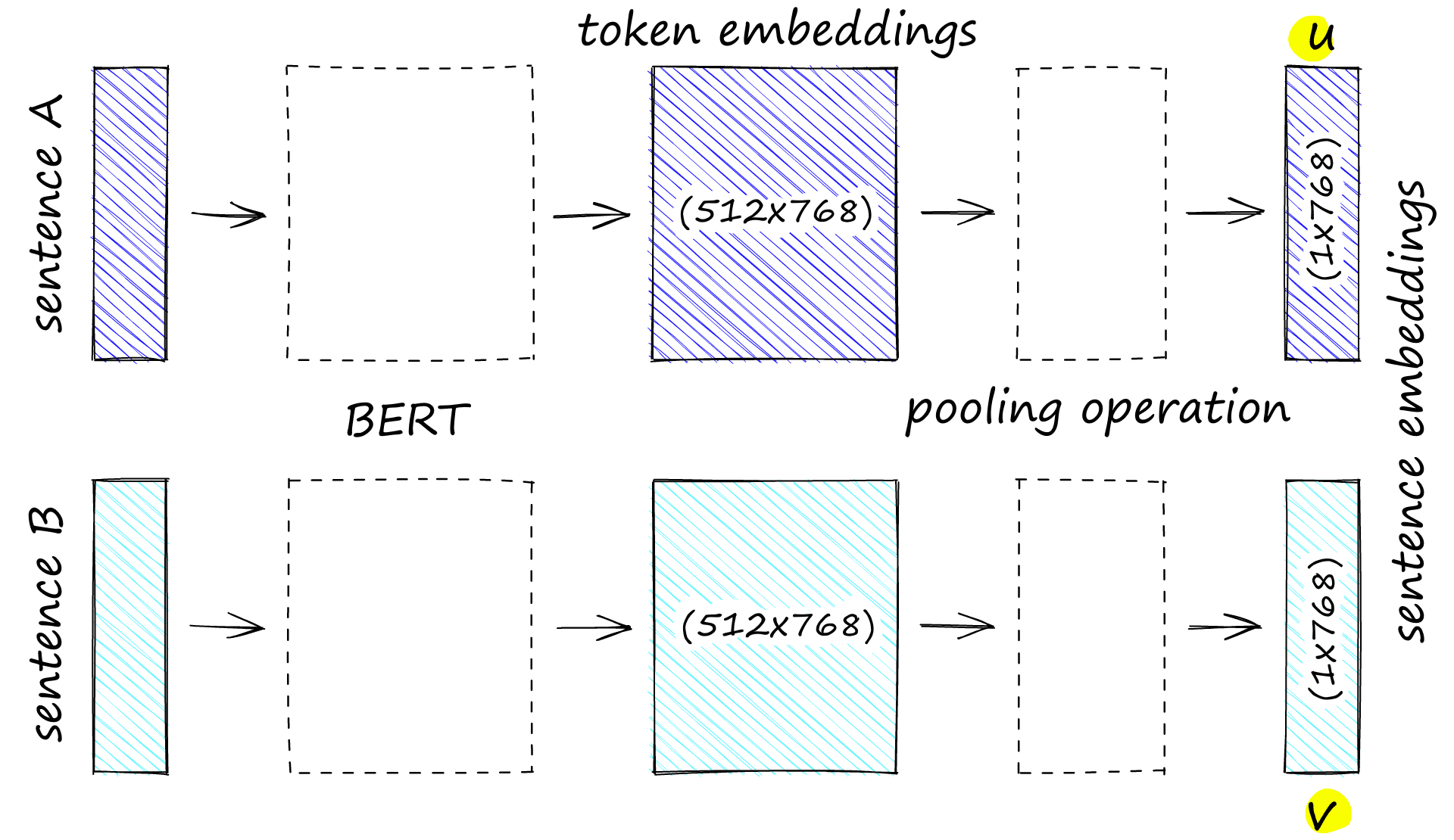
Siamese-BERT processing a sentence pair and then pooling the large token embeddings tensor into a single dense vector.
BERT will output 512 768-dimensional embeddings. We will convert these into an average embedding using mean-pooling. This pooled output is our sentence embedding. We will have two per step — one for sentence A that we call u, and one for sentence B, called v.
To perform this mean pooling operation, we will define a function called mean_pool.
# define mean pooling function
def mean_pool(token_embeds, attention_mask):
    # reshape attention_mask to cover 768-dimension embeddings
    in_mask = attention_mask.unsqueeze(-1).expand(
        token_embeds.size()
    ).float()
    # perform mean-pooling but exclude padding tokens (specified by in_mask)
    pool = torch.sum(token_embeds * in_mask, 1) / torch.clamp(
        in_mask.sum(1), min=1e-9
    )
    return pool
Here we take BERT’s token embeddings output (we’ll see this all in full soon) and the sentence’s attention_mask tensor. We then resize the attention_mask to align to the higher 768-dimensionality of the token embeddings.
We apply this resized mask in_mask to those token embeddings to exclude padding tokens from the mean pooling operation. Our mean pooling takes the average activation of values across each dimension to produce a single value. This brings our tensor sizes from (512*768) to (1*768).
The next step is to concatenate these embeddings. Several different approaches to this were presented in the paper:
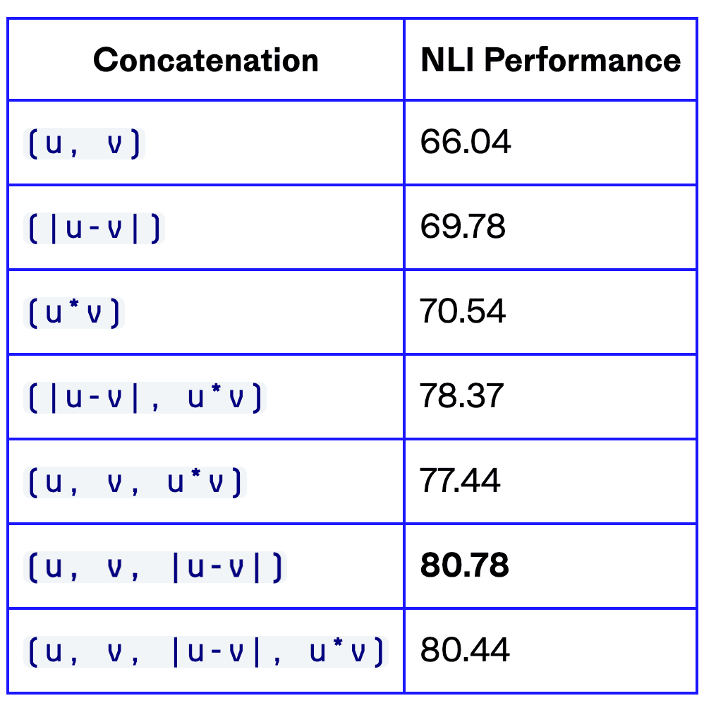
Concatenation methods for sentence embeddings u and v and their performance on STS benchmarks.
Of these, the best performing is built by concatenating vectors u, v, and |u-v|. Concatenation of them all produces a vector three times the length of each original vector. We label this concatenated vector (u, v, |u-v|). Where |u-v| is the element-wise difference between vectors u and v.
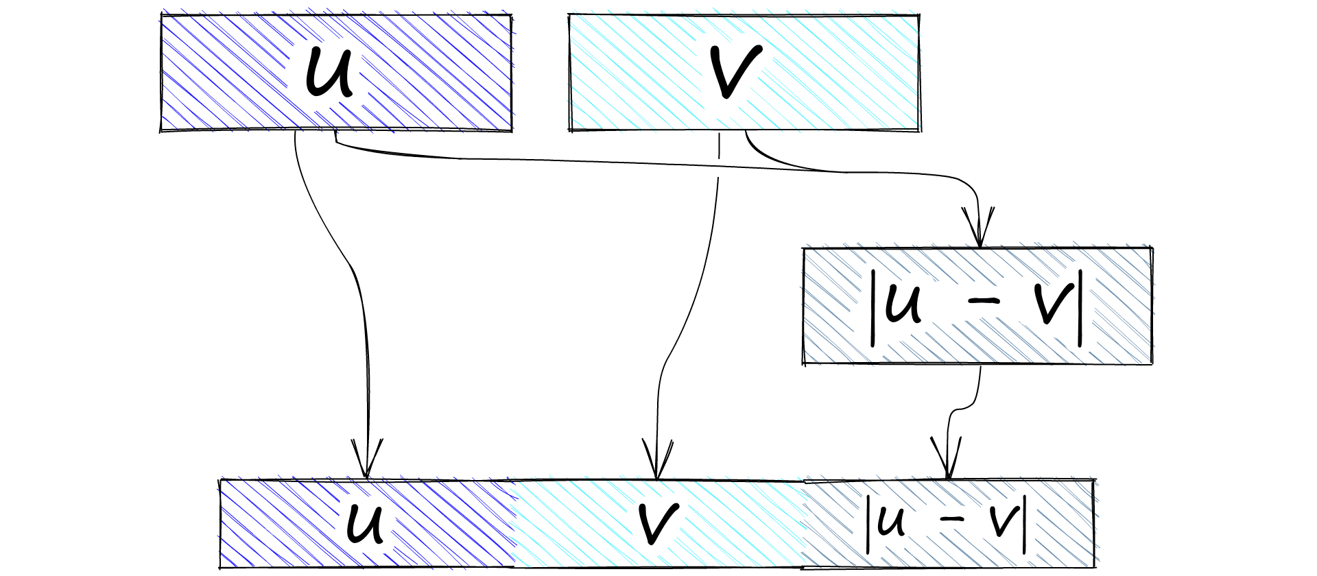
We concatenate (u, v, |u-v|) to merge the sentence embeddings from sentence A and B.
We will perform this concatenation operation using PyTorch. Once we have our mean-pooled sentence vectors u and v we concatenate with:
uv_abs = torch.abs(torch.sub(u, v))  # produces |u-v| tensor
# then we concatenate
x = torch.cat([u, v, uv_abs], dim=-1)
Vector (u, v, |u-v|) is fed into a feed-forward neural network (FFNN). The FFNN processes the vector and outputs three activation values. One for each of our label classes; entailment, neutral, and contradiction.
# we would initialize the feed-forward NN first
ffnn = torch.nn.Linear(768*3, 3)
	...
# then later in the code process our concatenated vector with it
x = ffnn(x)
As these activations and label classes are aligned, we now calculate the softmax loss between them.
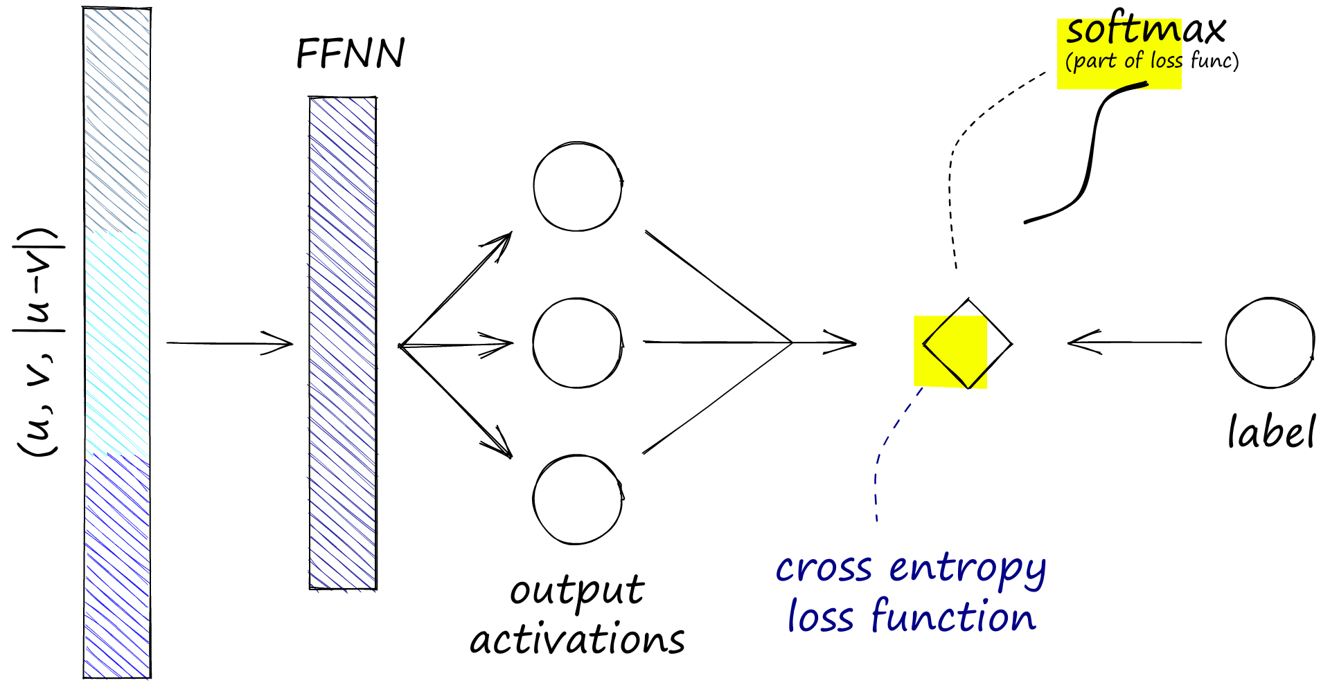
The final steps of training. The concatenated (u, v, |u-v|) vector is fed through a feed-forward NN to produce three output activations. Then we calculate the softmax loss between these predictions and the true labels.
Softmax loss is calculated by applying a softmax function across the three activation values (or nodes), producing a predicted label. We then use cross-entropy loss to calculate the difference between our predicted label and true label.
# as before, we would initialize the loss function first
loss_func = torch.nn.CrossEntropyLoss()
	...
# then later in the code add them to the process
x = loss_func(x, label)  # label is our *true* 0, 1, 2 class
The model is then optimized using this loss. We use an Adam optimizer with a learning rate of 2e-5 and a linear warmup period of 10% of the total training data for the optimization function. To set that up, we use the standard PyTorch Adam optimizer alongside a learning rate scheduler provided by HF transformers:
from transformers.optimization import get_linear_schedule_with_warmup

# we would initialize everything first
optim = torch.optim.Adam(model.parameters(), lr=2e-5)
# and setup a warmup for the first ~10% steps
total_steps = int(len(dataset) / batch_size)
warmup_steps = int(0.1 * total_steps)
scheduler = get_linear_schedule_with_warmup(
		optim, num_warmup_steps=warmup_steps,
  	num_training_steps=total_steps - warmup_steps
)
	...
# then during the training loop we update the scheduler per step
scheduler.step()
Now let’s put all of that together in a PyTorch training loop.
In[18]:
from tqdm.auto import tqdm

# 1 epoch should be enough, increase if wanted
for epoch in range(1):
    model.train()  # make sure model is in training mode
    # initialize the dataloader loop with tqdm (tqdm == progress bar)
    loop = tqdm(loader, leave=True)
    for batch in loop:
        # zero all gradients on each new step
        optim.zero_grad()
        # prepare batches and more all to the active device
        inputs_ids_a = batch['premise_input_ids'].to(device)
        inputs_ids_b = batch['hypothesis_input_ids'].to(device)
        attention_a = batch['premise_attention_mask'].to(device)
        attention_b = batch['hypothesis_attention_mask'].to(device)
        label = batch['label'].to(device)
        # extract token embeddings from BERT
        u = model(
            inputs_ids_a, attention_mask=attention_a
        )[0]  # all token embeddings A
        v = model(
            inputs_ids_b, attention_mask=attention_b
        )[0]  # all token embeddings B
        # get the mean pooled vectors
        u = mean_pool(u, attention_a)
        v = mean_pool(v, attention_b)
        # build the |u-v| tensor
        uv = torch.sub(u, v)
        uv_abs = torch.abs(uv)
        # concatenate u, v, |u-v|
        x = torch.cat([u, v, uv_abs], dim=-1)
        # process concatenated tensor through FFNN
        x = ffnn(x)
        # calculate the 'softmax-loss' between predicted and true label
        loss = loss_func(x, label)
        # using loss, calculate gradients and then optimize
        loss.backward()
        optim.step()
        # update learning rate scheduler
        scheduler.step()
        # update the TDQM progress bar
        loop.set_description(f'Epoch {epoch}')
        loop.set_postfix(loss=loss.item())
Out[18]:
Epoch 0: 100%|██████████| 58880/58880 [2:37:36<00:00, 6.23it/s, loss=0.876]
We only train for a single epoch here. Realistically this should be enough (and mirrors what was described in the original SBERT paper). The last thing we need to do is save the model.
In[19]:
import os

model_path = './sbert_test_a'

if not os.path.exists(model_path):
    os.mkdir(model_path)

model.save_pretrained(model_path)
Now let’s compare everything we’ve done so far with sentence-transformers training utilities. We will compare this and other sentence transformer models at the end of the article.
Fine-Tuning With Sentence Transformers
As we already mentioned, the sentence-transformers library has excellent support for those of us just wanting to train a model without worrying about the underlying training mechanisms.
We don’t need to do much beyond a little data preprocessing (but less than what we did above). So let’s go ahead and put together the same fine-tuning process, but using sentence-transformers.
Training Data
Again we’re using the same SNLI and MNLI corpora, but this time we will be transforming them into the format required by sentence-transformers using their InputExample class. Before that, we need to download and merge the two datasets just like before.
In[1]:
import datasets

# download
snli = datasets.load_dataset('snli', split='train')
mnli = datasets.load_dataset('glue', 'mnli', split='train')

# format for merge
mnli = mnli.remove_columns(['idx'])
snli = snli.cast(mnli.features)

# merge
nli = datasets.concatenate_datasets([snli, mnli])
del snli, mnli

# and remove bad rows
nli = nli.filter(
    lambda x: False if x['label'] == -1 else True
)
Out[1]:
Reusing dataset snli
Reusing dataset glue
100%|██████████| 56/56 [00:01<00:00, 51.32ba/s]
100%|██████████| 943/943 [00:18<00:00, 51.48ba/s]
Now we’re ready to format our data for sentence-transformers. All we do is convert the current premise, hypothesis, and label format into an almost matching format with the InputExample class.
In[2]:
from sentence_transformers import InputExample
from tqdm.auto import tqdm  # so we see progress bar

train_samples = []
for row in tqdm(nli):
    train_samples.append(InputExample(
        texts=[row['premise'], row['hypothesis']],
        label=row['label']
    ))
Out[2]:
100%|██████████| 942069/942069 [00:33<00:00, 28240.15it/s]
In[3]:
from torch.utils.data import DataLoader

batch_size = 16

loader = DataLoader(
    train_samples, shuffle=True, batch_size=batch_size)
We’ve also initialized a DataLoader just as we did before. From here, we want to begin setting up the model. In sentence-transformers we build models using different modules.
All we need is the transformer model module, followed by a mean pooling module. The transformer models are loaded from HF, so we define bert-base-uncased as before.
In[4]:
from sentence_transformers import models, SentenceTransformer

bert = models.Transformer('bert-base-uncased')
pooler = models.Pooling(
    bert.get_word_embedding_dimension(),
    pooling_mode_mean_tokens=True
)

model = SentenceTransformer(modules=[bert, pooler])

model
Out[4]:
SentenceTransformer(
  (0): Transformer({'max_seq_length': 512, 'do_lower_case': False}) with Transformer model: BertModel
  (1): Pooling({'word_embedding_dimension': 768, 'pooling_mode_cls_token': False, 'pooling_mode_mean_tokens': True, 'pooling_mode_max_tokens': False, 'pooling_mode_mean_sqrt_len_tokens': False})
)
Now we’re ready to train the model. We train for a single epoch and warm up for 10% of training as before.
In[6]:
epochs = 1
warmup_steps = int(len(loader) * epochs * 0.1)

model.fit(
    train_objectives=[(loader, loss)],
    epochs=epochs,
    warmup_steps=warmup_steps,
    output_path='./sbert_test_b',
    show_progress_bar=False,
)
With that, we’re done, the new model is saved to ./sbert_test_b. We can load the model from that location using either the SentenceTransformer or HF’s from_pretrained methods! Let’s move on to comparing this to other SBERT models.
Compare SBERT Models
We’re going to test the models on a set of random sentences. We will build our mean-pooled embeddings for each sentence using four models; softmax-loss SBERT, multiple-negatives-ranking-loss SBERT, the original SBERT sentence-transformers/bert-base-nli-mean-tokens, and BERT bert-base-uncased.
sentences = [
    "the fifty mannequin heads floating in the pool kind of freaked them out",
    "she swore she just saw her sushi move",
    "he embraced his new life as an eggplant",
    "my dentist tells me that chewing bricks is very bad for your teeth",
    "the dental specialist recommended an immediate stop to flossing with construction materials",
    "i used to practice weaving with spaghetti three hours a day",
    "the white water rafting trip was suddenly halted by the unexpected brick wall",
    "the person would knit using noodles for a few hours daily",
    "it was always dangerous to drive with him since he insisted the safety cones were a slalom course",
    "the woman thinks she saw her raw fish and rice change position"
]
After producing sentence embeddings, we will calculate the cosine similarity between all possible sentence pairs, producing a simple but insightful semantic textual similarity (STS) test.
We define two new functions; sts_process to build the sentence embeddings and compare them with cosine similarity and sim_matrix to construct a similarity matrix from all possible pairs.
import numpy as np

# build embeddings and calculate cosine similarity
def sts_process(sentence_a, sentence_b, model):
    vecs = []  # init list of sentence vecs
    for sentence in [sentence_a, sentence_b]:
        # build input_ids and attention_mask tensors with tokenizer
        input_ids = tokenizer(
            sentence, max_length=512, padding='max_length',
            truncation=True, return_tensors='pt'
        )
        # process tokens through model and extract token embeddings
        token_embeds = model(**input_ids).last_hidden_state
        # mean-pool token embeddings to create sentence embeddings
        sentence_embeds = mean_pool(token_embeds, input_ids['attention_mask'])
        vecs.append(sentence_embeds)
    # calculate cosine similarity between pairs and return numpy array
    return cos_sim(vecs[0], vecs[1]).detach().numpy()

# controller function to build similarity matrix
def sim_matrix(model):
    # initialize empty zeros array to store similarity scores
    sim = np.zeros((len(sentences), len(sentences)))
    for i in range(len(sentences)):
        # add similarity scores to the similarity matrix
        sim[i:,i] = sts_process(sentences[i], sentences[i:], model)
    return sim
Then we just run each model through the sim_matrix function.
import matplotlib.pyplot as plt
import seaborn as sns

tokenizer = BertTokenizer.from_pretrained('bert-base-uncased')
model = BertModel.from_pretrained('./sbert_test_a')

sim = sim_matrix(model)  # build similarity scores matrix
sns.heatmap(sim, annot=True)  # visualize heatmap
After processing all pairs, we visualize the results in heatmap visualizations.
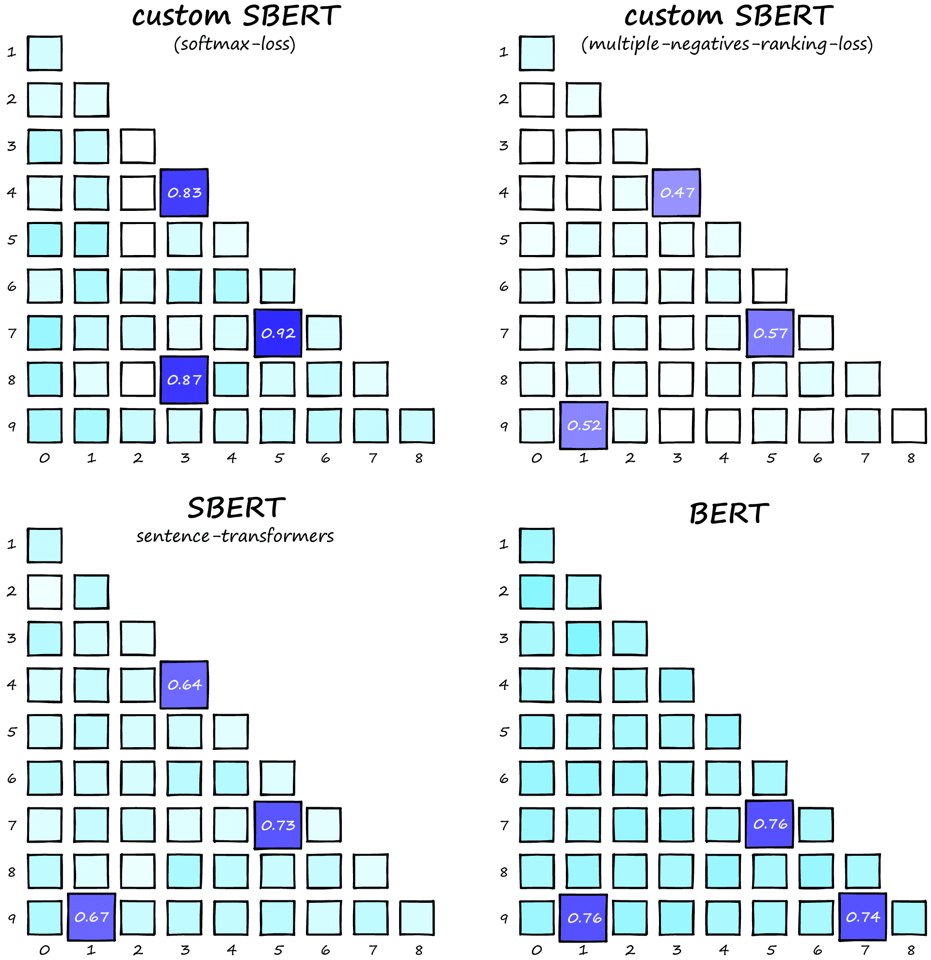
Similarity score heatmaps for four BERT/SBERT models.
Similarity score heatmaps for four BERT/SBERT models.
In these heatmaps, we ideally want all dissimilar pairs to have very low scores (near white) and similar pairs to produce distinctly higher scores.
Let’s talk through these results. The bottom-left and top-right models produce the correct top three pairs, whereas BERT and softmax loss SBERT return 2/3 of the correct pairs.
If we focus on the standard BERT model, we see minimal variation in square color. This is because almost every pair produces a similarity score of between 0.6 to 0.7. This lack of variation makes it challenging to distinguish between more-or-less similar pairs. Although this is to be expected as BERT has not been fine-tuned for semantic similarity.
Our PyTorch softmax loss SBERT (top-left) misses the 9-1 sentence pair. Nonetheless, the pairs it produces are much more distinct from dissimilar pairs than the vanilla BERT model, so it’s an improvement. The sentence-transformers version is better still and did not miss the 9-1 pair.
Next up, we have the SBERT model trained by Reimers and Gurevych in the 2019 paper (bottom-left) [1]. It produces better performance than our SBERT models but still has little variation between similar and dissimilar pairs.
And finally, we have an SBERT model trained using MNR loss. This model is easily the highest performing. Most dissimilar pairs produce a score very close to zero. The highest non-pair returns 0.28 — roughly half of the true-pair scores.
From these results, the SBERT MNR model seems to be the highest performing. Producing much higher activations (with respect to the average) for true pairs than any other model, making similarity much easier to identify. SBERT with softmax loss is clearly an improvement over BERT, but unlikely to offer any benefit over the SBERT with MNR loss model.
That’s it for this article on fine-tuning BERT for building sentence embeddings! We delved into the details of preprocessing SNLI and MNLI datasets for NLI training and how to fine-tune BERT using the softmax loss approach.
Finally, we compared this softmax-loss SBERT against vanilla BERT, the original SBERT, and an MNR loss SBERT using a simple STS task. We found that although fine-tuning with softmax loss does produce valuable sentence embeddings — it still lacks quality compared to more recent training approaches.
We hope this has been an insightful and exciting exploration of how transformers can be fine-tuned for building sentence embeddings.
References
[1] N. Reimers, I. Gurevych, Sentence-BERT: Sentence Embeddings using Siamese BERT-Networks (2019), ACL
Was this article helpful?