In computer vision, bag of visual words (BoVW) is one of the pre-deep learning methods used for building image embeddings. We can use BoVW for content-based image retrieval, object detection, and image classification.

At a high level, comparing images with the bag of visual words approach consists of five steps:

1. Extract visual features,
2. Create visual words,
3. Build sparse frequency vectors with these visual words,
4. Adjust frequency vectors for relevant with tf-idf,
5. Compare vectors with similarity or distance metrics.

We will start by walking through the theory of how all of this works. In the second half of this article we will look at how to implement all of this in Python.

How Bag of Visual Words Works

Visual Features

The model derives from bag of words in natural language processing (NLP), where a chunk of text is split into words or sub-words and those components are collated into an unordered list, the so-called “bag of words” (BoW).

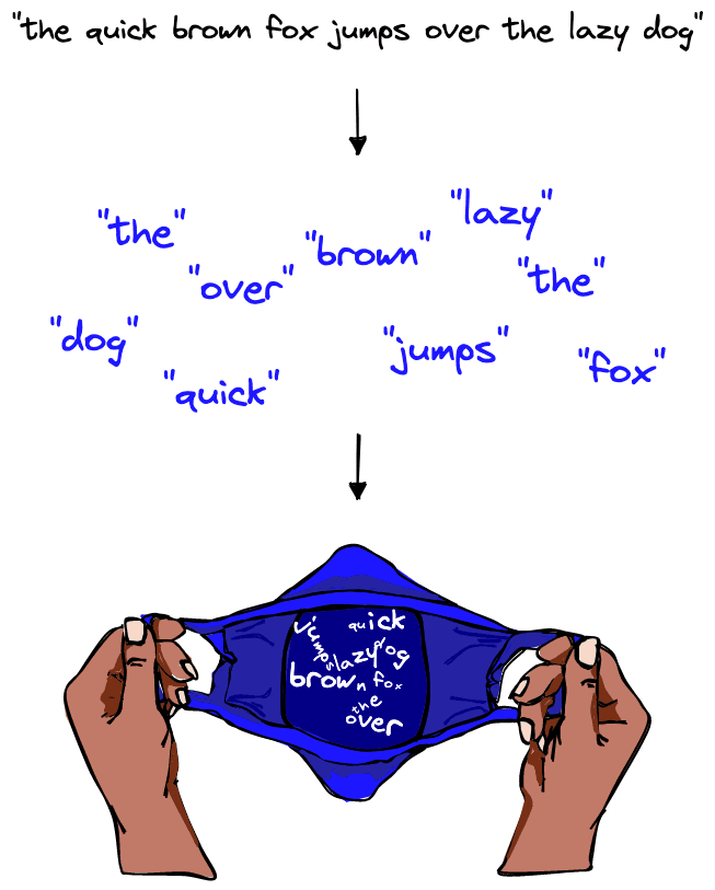
Similarly, in bag of visual words the images are represented by patches, and their unique patterns (or visual features) are extracted from the image.

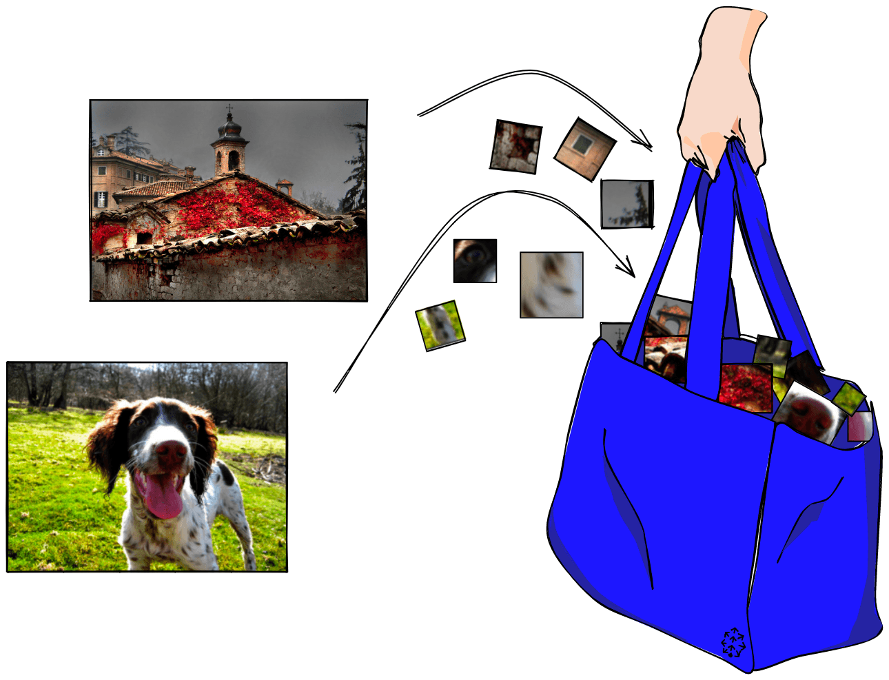
However, despite the similarity, these visual features are not visual words just yet; we must perform a few more steps. For now, let’s focus on understanding what these visual features are.

Visual features consist of two items:

• Keypoints are points in an image, which do not change if the image is rotated, expanded, or scaled and
• Descriptors are vector representations of an image patch found at a given keypoint.

These visual features can be detected and extracted using a feature detector, such as SIFT (Scale Invariant Feature Transform), ORB (Oriented FAST and Rotated BRIEF), or SURF (Speeded Up Robust Features).

The most common is SIFT as it is invariant to scale, rotation, translation, illumination, and blur. SIFT converts each image patch into a 128128-dimensional vector (i.e., the descriptor of the visual feature).

A single image will be represented by many SIFT vectors. The order of these vectors is not important, only their presence within an image.

Codebooks and Visual Words

After extracting visual features we build a codebook, also called a dictionary or vocabulary. This codebook acts as a repository of all existing visual words (similar to an actual dictionary, like the Oxford English Dictionary).

We use this codebook as a way to translate a potentially infinite variation of visual features into a predefined set of visual words.

How? The idea is to group similar visual features into clusters. Each cluster is assigned a central point which represents the visual word translation (or mapping) for that group of visual features. The standard approach for grouping visual features into visual words is k-means clustering.

K-means divides the data into clusters, where is chosen by us. Once the data is grouped, k-means calculates the mean for each cluster, i.e., a central point between all of the vectors in a group. That central point is a centroid (i.e., a visual word).

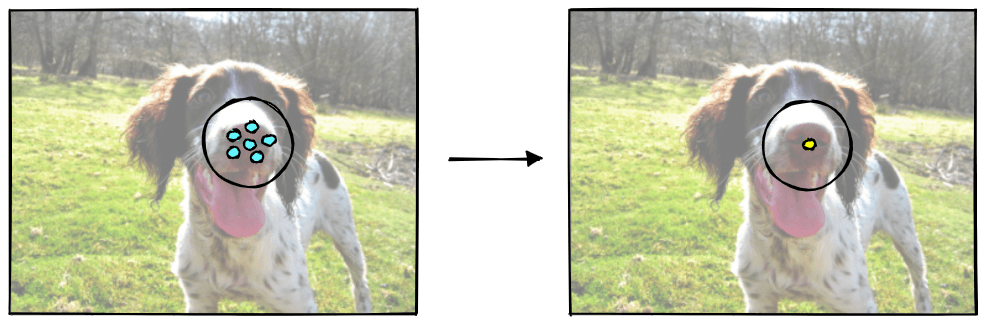
After finding the centroids, k-means iterates through each data point (visual feature) and checks which centroid (visual word) is nearest. If the nearest centroid has changed, the data point switches grouping, being assigned to the new nearest centroid.

This process is repeated over a given number of iterations or until the centroid positions have stabilized.

With that in mind, how do we choose the number of centroids, ?

It is more of an art than a science, but there are a few things to consider. Primarily, how many visual words can cover the various relevant visual features in the dataset.

That’s not an easy thing to figure out, and it’s always going to require some guesswork. However, we can think of it using the language equivalent, bag of words.

If our language dataset covered several documents about a specific topic in a single language, we would find fewer unique words than if we had thousands of documents, spanning several languages about a range of topics.

The same is true for images; dogs and/or animals could be a topic, and buildings could be another topic. As for the equivalent of different languages, this is not a perfect metaphor but we could think of different photography styles, drawings, or cartoons. All of these added layers of complexity increase the number of visual words needed to accurately represent the dataset.

Here, we could start with choosing a smaller value (e.g., 100100 or 150150) and re-run the code multiple times changing until convergence and/or our model seems to be identifying images well.

If we choose =150=150, k-means will generate 150150 centroids and, therefore, 150150 visual words.

When we perform the mapping from new visual feature vectors to the nearest centroid (i.e., visual word), we categorize visual features into a more limited set of visual words. This process of reducing the number of possible unique vectors is called vector quantization.

Using a limited set of visual words allows us to compress our image descriptions into a set of visual word IDs. And, more importantly, it helps us represent similar features across images using a shared set of visual words.

That means that the visual words shared by two images of churches may be quite large, meaning they’re similar. However, an image of a church and an image of a dog will share far fewer visual words, meaning they’re dissimilar.

After those steps, our images will be represented by a varying number of visual words. From here we move on to the next step of transforming these visual words into image-level frequency vectors.

Frequency Vectors

We can count the frequency of these visual words and visualize them with histograms.

The x-axis of the histogram is the codebook, while the y-axis is the frequency of each visual word (in the codebook) for that image.

If we consider 22 images, we can represent the image histograms as follows:

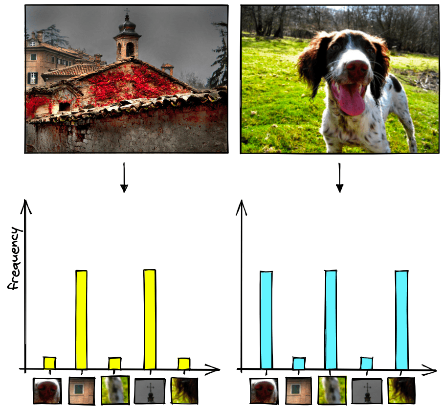
To create these representations, we have converted each image into a sparse vector where each value in the vector represents an item in the codebook (i.e., the x-axis in the histograms). Most of the values in each vector will be zero because most images will only contain a small percentage of total number of visual words, which is why we refer to them as sparse vectors.

As for the non-zero values in our sparse vector, they are calculated in the same way that we calculated our histogram bar heights. They are equal to the frequency of a particular visual word in an image.

This works, but it’s a crude way to create these sparse vector representations. Because many visual words are actually not that important, we add one more step.

Tf-idf

In language there are some words that are more important than others in that they give us more information. If we used the sentence “the history of Rome” to search through a set of articles, the words “the” and “of” should not be given the same importance as “history” or “Rome”.

These less important words are often very common. If we only consider the frequency of words shared with our “the history of Rome” query, the article with the most “the"s could be scored highest.

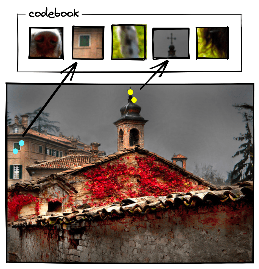
This problem is also found in images. A visual word extracted from a patch of sky in an image is unlikely to tell us whether this image is of a church or a dog. Some visual words are more relevant than others.

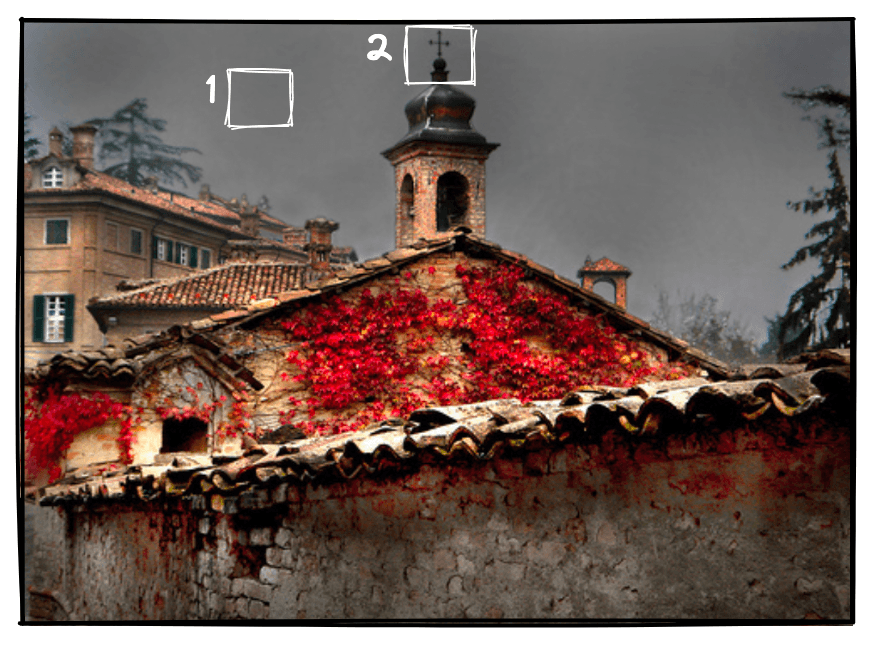
In the example above, we would expect a visual word representing the sky 1 to be less relevant than a visual word representing the cross on top of the bell tower 2.

That is why it is important to adjust the values of our sparse vector to give more weight to more relevant visual words and less weight to less relevant visual words.

To do that, we can use the tf-idf (term-frequency inverse document frequency) formula, which is calculated as follows:

Where:

• is the term frequency of the visual word in the image (the number of times occurs in ),
• is the total number of images,
• number of images containing visual word ,
• measures how common the visual word is across all images in the database. This is low if the visual word occurs many times in the image, high otherwise.

After tf-idf, we can visualize the vectors via our histogram again, which will better reflect the image’s features.

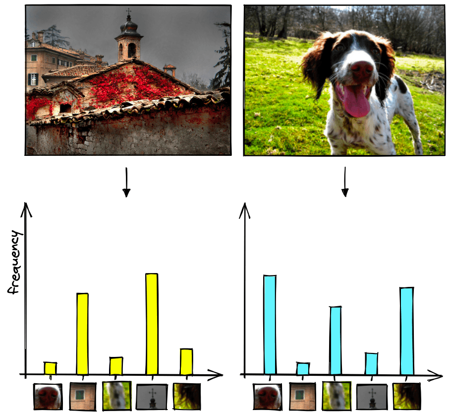
Before we were giving the same importance to image’s patches in an image; now they’re adjusted based on relevance and then normalized.

We’ve now trained our codebook and learned how to process each vector for better relevance and normalization. When wanting to embed new images with this pipeline, we repeat the process but avoid retraining the codebook. Meaning we:

1. Extract the visual features,
2. Transform them into visual words using the existing codebook,
3. Use these visual words to create a sparse frequency vector,
4. Adjust the frequency vector based on relevance with tf-idf, giving us our final sparse vector representations.

After that, we’re ready to compare these sparse vectors to find similar or dissimilar images.

Measuring Similarity

There are several metrics we can use to calculate similarity or distance between two vectors. The most common are:

1. Cosine similarity,
2. Euclidean distance, and
3. Dot product similarity.

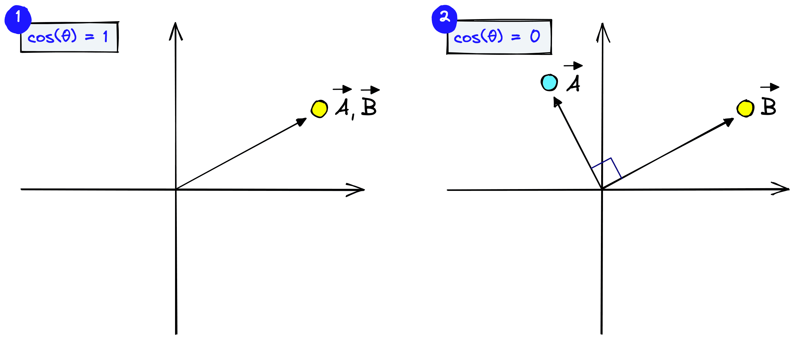
We will use cosine similarity which measures the angle between vectors. Vectors pointing in a similar direction have a lower angular separation and therefore higher cosine similarity.

Cosine similarity is calculated as:

Cosine similarity generally gives a value ranging [−1,1]. However, if we think about the frequency of visual words, we cannot consider them as negative. Therefore, the angle between two term frequency vectors cannot be greater than 90°, and cosine similarity ranges between [0,1].

It equals 1 if the vectors are pointing in the same direction (the angle equals 0) and 0 if vectors are perpendicular.

If we consider three different images and we build a matrix based on cosine similarity:

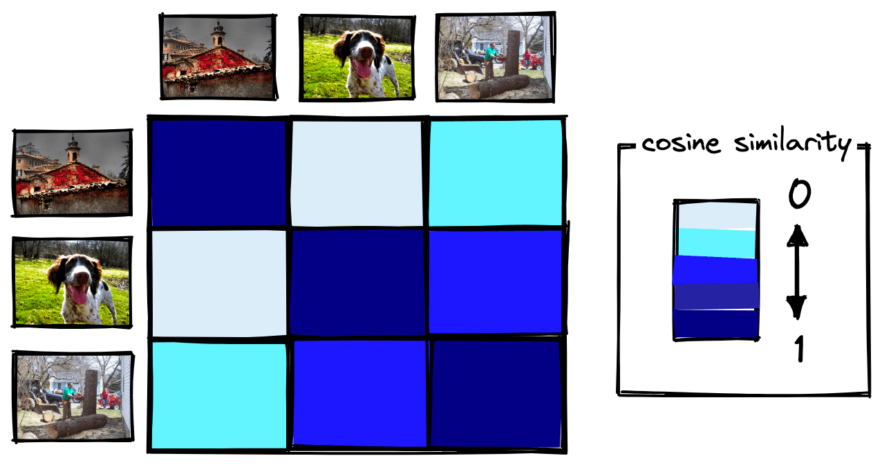
We can see that cosine similarity is 11 when the image is exactly the same (i.e., in the main diagonal). The cosine similarity approaches 00 as the images have less in common.

Let’s now move on to implementing bag of visual words with Python.

Implementing Bag of Visual Words

The next section will work through the implementation of everything we’ve just learned in Python. If you’d like to follow along, use this code notebook.

Imagenette Dataset Preprocessing

First, we want to import a dataset of images to train the model.

Feel free to use any images you like. However, if you’d like to follow along with the same dataset, we will use the frgfm/imagenette dataset from HuggingFace Datasets.

from datasets import load_dataset

# download the dataset
imagenet = load_dataset(
    'frgfm/imagenette',
    'full_size',
    split='train',
    ignore_verifications=False  # set to True if seeing splits Error
)
imagenet

Dataset({
    features: ['image', 'label'],
    num_rows: 9469
})

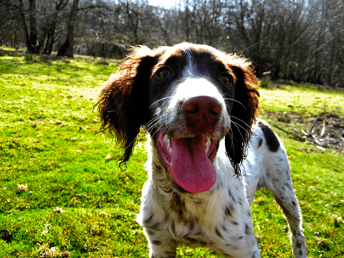
The dataset contains 9469 images, covering a range of images with dogs, radios, fishing, cities, etc. The image feature contains the images themselves stored as PIL object, meaning we can view them in a notebook like so:

# important to use imagenet[0]['image'] rather than imagenet['image'][0]
# as the latter loads the entire image column then extracts index 0 (it's slow)
imagenet[3264]['image']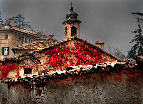

To process these images we need to transform them from PIL objects to numpy arrays.

import numpy as np

# initialize list
images_training = []

for n in range(0,len(imagenet)):
    # generate np arrays from the dataset images
    images_training.append(np.array(imagenet[n]['image']))

The dataset mostly consists of color images containing three color channels (red, green, and blue), but some are also grayscale containing just a single channel (brightness). To optimize processing time and keep everything as simple as possible, we will transform color images to grayscale.

import cv2  # pip install opencv-contrib-python opencv-python

# convert images to grayscale
bw_images = []
for img in images_training:
    # if RGB, transform into grayscale
    if len(img.shape) == 3:
        bw_images.append(cv2.cvtColor(img, cv2.COLOR_BGR2GRAY))
    else:
        # if grayscale, do not transform
        bw_images.append(img)

The arrays in bw_images are what we will be using to create our visual features, visual words, frequency vectors, and tf-idf vectors.

Visual Features

With our dataset prepared we’re ready to move on to extracting visual features (both keypoints and descriptors). As mentioned earlier, we will use the SIFT feature detection algorithm.

# defining feature extractor that we want to use (SIFT)
extractor = cv2.xfeatures2d.SIFT_create()

# initialize lists where we will store *all* keypoints and descriptors
keypoints = []
descriptors = []

for img in bw_images:
    # extract keypoints and descriptors for each image
    img_keypoints, img_descriptors = extractor.detectAndCompute(img, None)
    keypoints.append(img_keypoints)
    descriptors.append(img_descriptors)

It’s worth noting that if an image doesn’t have any noticeable features (e.g., it is a flat image without any edges, gradients, etc.), extraction with SIFT can return None. We don’t have that problem with this dataset, but it’s something to watch out for with others.

Now that we have extracted the visual features, we can visualize them with matplotlib.

output_image = []
for x in range(3):
    output_image.append(cv2.drawKeypoints(bw_images[x], keypoints[x], 0, (255, 0, 0),
                                 flags=cv2.DRAW_MATCHES_FLAGS_DRAW_RICH_KEYPOINTS))
    plt.imshow(output_image[x], cmap='gray')
    plt.show()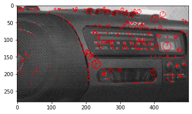

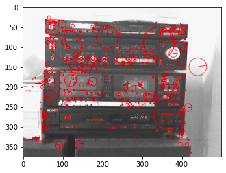
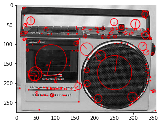
The centre of each circle is the keypoint location, and the lines from the centre of each circle represent keypoint orientation. The size of each circle is the scale at which the features were detected.

With our visual features ready, we can move onto the next step of creating visual words.

Visual Words and the Codebook

Earlier we described the “codebook”. The codebook acts as a vocabulary where we store all of our visual words. To create the codebook we use k-means clustering to quantize our visual features into a smaller set of visual words.

Our full set of visual features is big, and training k-means with the full set will take some time. So, to avoid that and also emulate a real-world scenario where we are unlikely to train on all images that we’ll ever process, we will use a smaller sample of 1000 images.

# set numpy seed for reproducability
np.random.seed(0)
# select 1000 random image index values
sample_idx = np.random.randint(0, len(imagenet)+1, 1000).tolist()

# extract the sample from descriptors
# (we don't need keypoints)
descriptors_sample = []

for n in sample_idx:
    descriptors_sample.append(np.array(descriptors[n]))

Our descriptors_sample contains a single array for each image, and each array can contain a varying number of SIFT feature vectors. When training k-means, we only care about the feature vectors, we don’t care about which image they’re coming from. So, we need to flatten descriptors_sample into a single array containing all descriptors.

all_descriptors = []
# extract image descriptor lists
for img_descriptors in descriptors_sample:
    # extract specific descriptors within the image
    for descriptor in img_descriptors:
        all_descriptors.append(descriptor)
# convert to single numpy array
all_descriptors = np.stack(all_descriptors)

# check the shape 
all_descriptors.shape

From this, we get all_descriptors, a single array containing all feature vectors from our sample. There are ~1.3M of these.

We now want to group similar visual features (descriptors) using k-means. After a few tests, we chose k=200 for our model.

After k-means, all images will have been reduced to visual words, and the full set of these visual words become our codebook.

# perform k-means clustering to build the codebook
from scipy.cluster.vq import kmeans

k = 200
iters = 1
codebook, variance = kmeans(all_descriptors, k, iters)

Once built, the codebook does not change. No matter how many more visual features we process, no more visual words are added as we will use it solely as a mapping between new visual features and the existing visual words.

It can be difficult to find the optimal size of our codebook - if too small, visual words could be unrepresentative of all image regions, and if too large, there could be too many visual words with little to no of them being shared between images (making comparisons very hard or impossible).

With our codebook complete, we can use it to transform the full dataset of visual features into visual words.

# vector quantization
from scipy.cluster.vq import vq

visual_words = []
for img_descriptors in descriptors:
    # for each image, map each descriptor to the nearest codebook entry
    img_visual_words, distance = vq(img_descriptors, codebook)
    visual_words.append(img_visual_words)

# let's see what the visual words look like for image 0
visual_words[0][:5], len(visual_words[0])

(array([ 84,  22,  45, 172, 172], dtype=int32), 397)

# the centroid that represents visual word 84 is of dimensionality...
codebook[84].shape  # (all have the same dimensionality)

We can see here that image 0 contains 397 visual words; the first five of those are represented by [84, 22, 45, 172, 172], which are the index values of the visual word vector found in the codebook. This visual word vector shares the same dimensionality as our SIFT feature vectors because it represents a cluster centroid from those feature vectors.

Sparse Frequency Vectors

After building our codebook and creating our image representations with visual words, we can move on to building sparse vector representations from these visual words.

We do this to compress the many visual word vectors representing our images into a single vector of set dimensionality. By doing this, we are able to directly compare our image representations using metrics like cosine similarity and Euclidean distance.

To create these frequency vectors, we look at how many times each visual word is found in an image. There are only 200 unique visual words (the length of our codebook), so each of these frequency vectors will have dimensionality 200, where each value becomes a count for a specific visual word.

frequency_vectors = []
for img_visual_words in visual_words:
    # create a frequency vector for each image
    img_frequency_vector = np.zeros(k)
    for word in img_visual_words:
        img_frequency_vector[word] += 1
    frequency_vectors.append(img_frequency_vector)
# stack together in numpy array
frequency_vectors = np.stack(frequency_vectors)

After creating the frequency vectors, we’re left with a single vector representation for each image. We can see an example of the frequency vector for image 0 below:

# we know from above that ids 84, 22, 45, and 172 appear in image 0
for i in [84,  22,  45, 172]:
    print(f"{i}: {frequency_vectors[0][i]}")

84: 2.0
22: 2.0
45: 3.0
172: 4.0

frequency_vectors[0][:20]

array([0., 0., 2., 0., 2., 1., 0., 3., 1., 0., 0., 0., 5., 3., 4., 0., 1.,
       0., 0., 0.])

# visualize the frequency vector for image 0
plt.bar(list(range(k)), frequency_vectors[0])
plt.show()

<Figure size 432x288 with 1 Axes>

Tf-idf

Our frequency vector can already be used for comparing images using our similarity and distance metrics. However, it is not ideal as it does not consider the different levels of relevance of each visual word. So, we must use tf-idf to adjust the frequency vector to consider relevance.

We first calculate and , both of which are shared across the entire dataset as the image is not considered by either parameter. Naturally, also produces a single vector shared by the full dataset.

# N is the number of images, i.e. the size of the dataset
N = 9469

# df is the number of images that a visual word appears in
# we calculate it by counting non-zero values as 1 and summing
df = np.sum(frequency_vectors > 0, axis=0)

((200,), array([7935, 7373, 7869, 8106, 7320]))

idf = np.log(N/ df)
idf.shape, idf[:5]

((200,), array([0.17673995, 0.25019863, 0.18509232, 0.15541878, 0.25741298]))

With calculated, we just need to multiply it by each vector to get our vectors. Fortunately, we already have the vectors, as they are our frequency vectors.

tfidf = frequency_vectors * idf
tfidf.shape, tfidf[0][:5]

((9469, 200),
 array([0.        , 0.        , 0.37018463, 0.        , 0.51482595]))

# we can visualize the histogram for image 0 again
plt.bar(list(range(k)), tfidf[0])
plt.show()

<Figure size 432x288 with 1 Axes>

We now have 9469 200-dimensional sparse vector representations of our images.

Search

These sparse vectors have been built in such a way that images that share many similar visual features should share similar sparse vectors. We can use cosine similarity to compare these images and identify similar images.

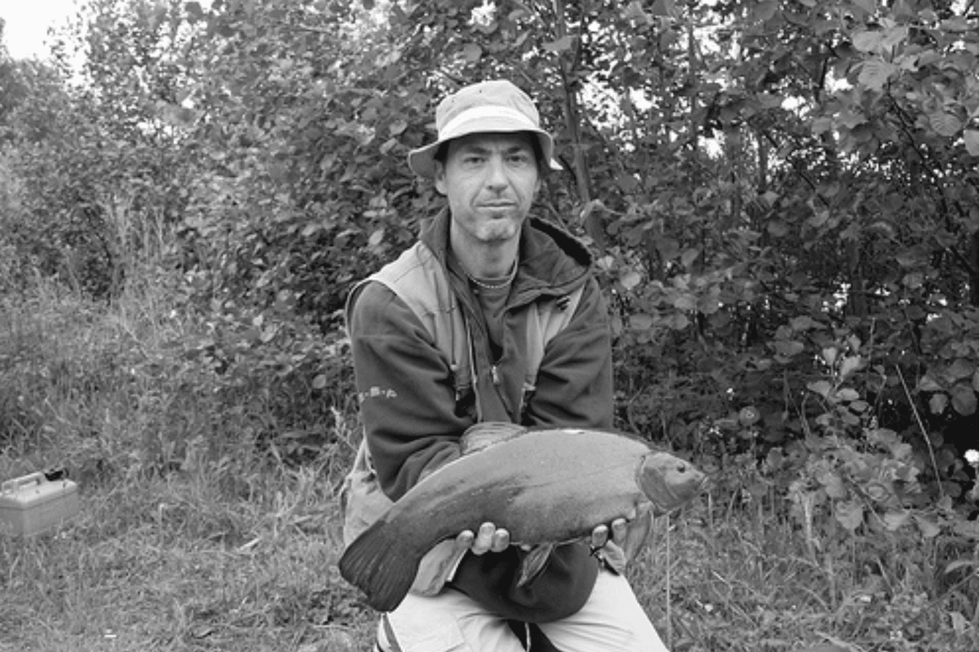
We will start by searching with image 1200:

from numpy.linalg import norm

top_k = 5
i = 1200

# get search image vector
a = tfidf[i]
b = tfidf  # set search space to the full sample
# get the cosine distance for the search image `a`
cosine_similarity = np.dot(a, b.T)/(norm(a) * norm(b, axis=1))
# get the top k indices for most similar vecs
idx = np.argsort(-cosine_similarity)[:top_k]
# display the results
for i in idx:
    print(f"{i}: {round(cosine_similarity[i], 4)}")
    plt.imshow(bw_images[i], cmap='gray')
    plt.show()

1200: 1.0

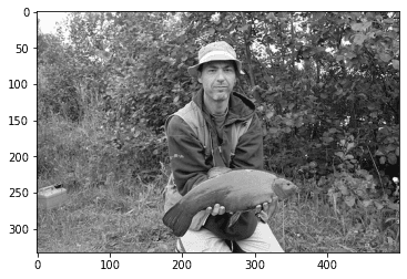
1609: 0.944

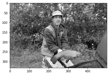
1739: 0.9397

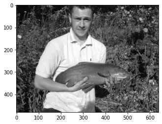
4722: 0.9346

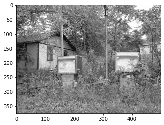
7381: 0.9304

The top image is of course the same image; as they are exact matches we can see the expected cosine similarity score of 1.0. Following this, we have two highly similar results. Interestingly, the fourth image seems to have been pulled through due to similarity in background foliage.

Here are a few more sets of results, showing the varied performance of the approach with different items.

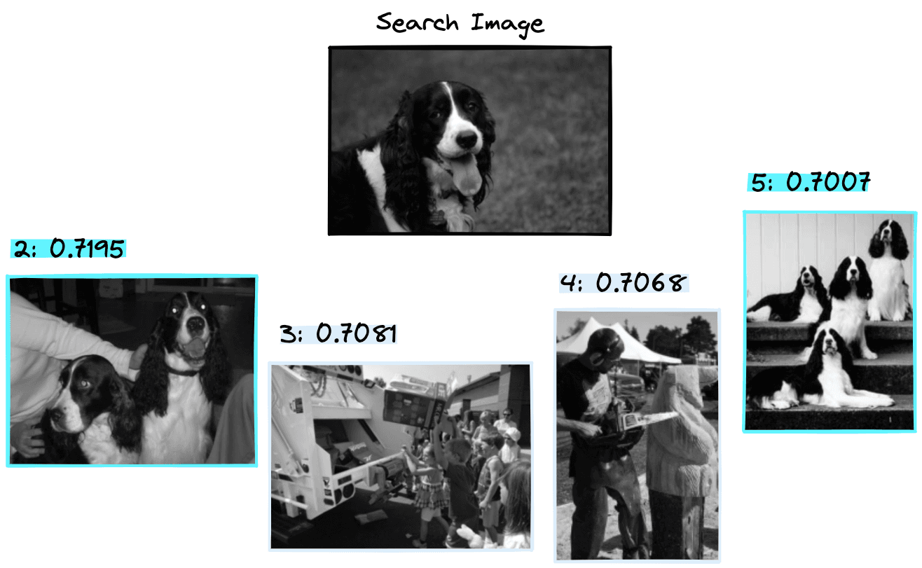
Here we get a good first result, followed by irrelevant images and a final good result in fifth position, a 50% success rate.

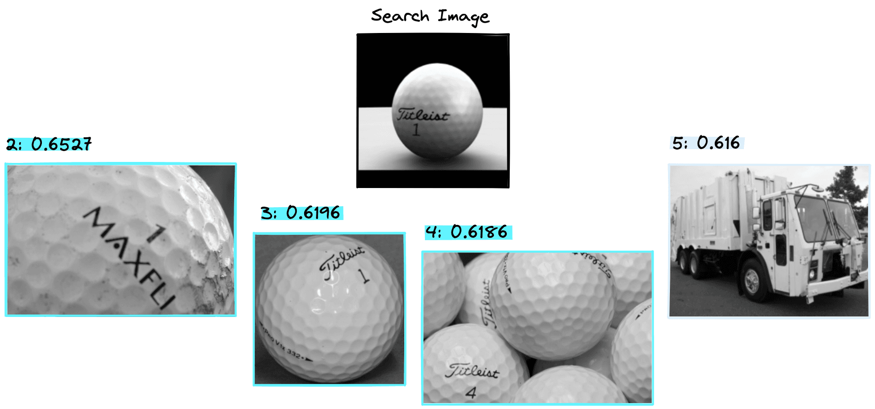
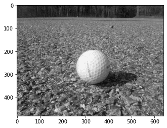
Bag of visual words seems to work well with golf balls, identifying 3/4 of relevant images.

If you’re interested in seeing more results, check out the Colab notebook here.

That’s it for this article on bag of visual words, one of the most successful methods for image classification and retrieval without the use of neural networks or other deep learning methods.

One great aspect of this approach is that it is fairly reliable and interpretable. There is no black box of AI here, so when applied to a lot of data we will rarely get too many surprising results.

We know that images with similar edges, textures, and colors are likely to be identified as similar; the features being identified are set by the SIFT (or other) algorithms.

All of this makes bag of visual words a good option for image retrieval or classification, where we need to focus on the features that we know algorithms like SIFT can deal with, i.e. we’re focused on finding similar object edges (that are resistant to scale, noise, and illumination changes). Finally, these well-defined algorithms give us a huge advantage when interpretability is important.

Resources

Code Notebook, GitHub Examples Repo