


In 1999, a concept known as the semantic web was described by the creator of the World Wide Web, Tim Berners-Lee. This dream of Berners-Lee was the internet of today that we know and love but deeply understood by machines [1].
This futuristic vision had seemed to be utterly infeasible, but, in recent years, has become much more than a dream. Thanks to techniques like Generative Pseudo-Labeling (GPL) that allow us to fine-tune new or existing models in previously inaccessible domains, machines are ever closer to understanding the meaning behind the content on the web.
I have a dream for the Web [in which computers] become capable of analyzing all the data on the Web – the content, links, and transactions between people and computers. A "Semantic Web", which makes this possible, has yet to emerge, but when it does, the day-to-day mechanisms of trade, bureaucracy and our daily lives will be handled by machines talking to machines. The "intelligent agents" people have touted for ages will finally materialize. - Tim Berners-Lee, 1999
Berners-Lee’s vision is fascinating, in particular the “intelligent agents” referred to in his quote above. Generally speaking, these intelligent agents (IAs) perceive their environment, take actions based on that environment to achieve a particular goal, and improve their performance with self-learning.
These IAs sound very much like the ML models we see today. Some models can look at a web page’s content (its environment), scrape and classify the meaning of this content (takes actions to achieve goals), and do this through an iterative learning process.
A model that can read and comprehend the meaning of language from the internet is a vital component of the semantic web. There are already models that can do this within a limited scope.
However, there is a problem. These Language Models (LMs) need to learn before becoming these autonomous, language-comprehending IAs. They must be trained.
Training LMs is hard; they need vast amounts of data. In particular, bi-encoder models (as explored in earlier chapters on AugSBERT and GenQ) that can enable a large chunk of this semantic web are notoriously data-hungry.
Sometimes this is okay. We can fine-tune a model easily in places where we have massive amounts of relevant and labeled data. We can use a simple supervised fine-tuning approach. Unfortunately, these scenarios are few and far between. It is for this reason that existing models have this limited scope. So, what can we do?
We should first consider why it is hard to get data to train these models. On one hand, the internet is full of data, and, on the other, this data is not in the format we need. We usually need to use a supervised training method to train a high-performance bi-encoder model.
Supervised training methods require labeled data. The problem with labeled data is that a human must (almost always) manually create it.
Currently, we have data-hungry models that require supervised training methods. We must find a way to train a model with little labeled data or use unsupervised methods that need nothing more than unstructured text data.
Fortunately, there are some unsupervised (or supervised using very little data) approaches, such as:
- Multilingual Knowledge Distillation for low-resource languages.
- TSDAE for building simple similarity models without labeled data.
- Data augmentation with AugSBERT for in-domain and out-of-domain tasks.
- GenQ for asymmetric semantic search without labeled data.
We can apply these approaches in different scenarios with varying degrees of success. As we’ve seen, there is a lot of potential for models being trained using unsupervised techniques. These no (or low) resource scenarios cover the vast majority of use-cases, many of which are the most unique and interesting.
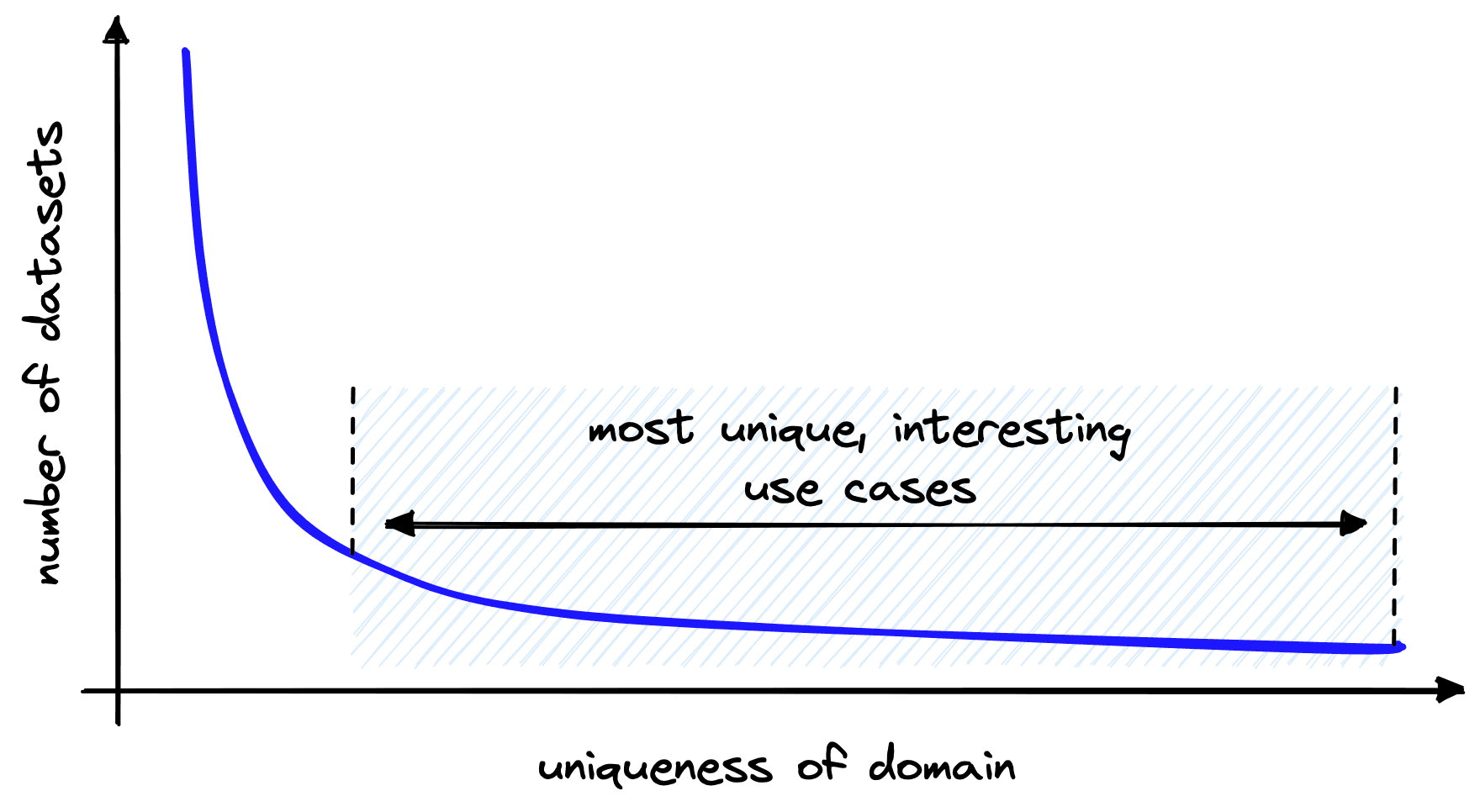
As the domain (eg topic, language) becomes more niche, the number of available labeled datasets decreases. The vast majority of domains have no labeled datasets.
For example, we may identify an opportunity to introduce semantic search on internal financial documents with highly technical language specific to our organization. Or a specific use-case using a less common language such as Swahili or Dhivehi.
It is infeasible for the semantic web to find labeled data for every topic, language, or format of information found on the internet. Because of this, the dream only becomes a reality once there are techniques that can train or adapt high-performance IAs with nothing more than the text found on the internet, without human-made labels or curation.
There is research producing techniques placing us ever closer to this reality. One of the most promising is GPL [2]. GPL is almost a culmination of the techniques listed above. At its core, it allows us to take unstructured text data and use it to build models that can understand this text. These models can then intelligently respond to natural language queries regarding this same text data.
It is a fascinating approach, with massive potential across innumerous use cases spanning all industries and borders. With that in mind, let’s dive into the details of GPL and how we can implement it to build high-performance LMs with nothing more than plain text.
Watch our webinar Searching Freely: Using GPL for Semantic Search for a rundown of GPL presented by Nils Reimers, the creator of sentence-transformers.
GPL Overview
GPL can be used in two ways, as a technique used in fine-tuning a pretrained model (such as the BERT base model), or as a technique for domain adaptation of an already fine-tuned bi-encoder model (such as SBERT).
By domain adaptation we mean the adaptation of an existing sentence transformer to new topics (domains). Effective domain adaptation is incredibly helpful in taking models pretrained on large, existing datasets, and helping them understand a new domain that lacks any labeled datasets.
For example, any model trained on data from before 2019 will be blissfully unaware of COVID-19 and everything that comes with it. If we query any of these pre-2019 models about COVID, they will struggle to return relevant information as they simply do not know what it is, and what is relevant.
In[13]:
show_examples(old_model)
# we can see similarity scores below
Out[13]:
Query: How is COVID-19 transmitted
94.83	Ebola is transmitted via direct contact with blood
92.86	HIV is transmitted via sex or sharing needles
92.31	Corona is transmitted via the air

Query: what is the latest named variant of corona
92.94	people keep drinking corona lager
91.91	the omicron variant of SARS-CoV-2
85.27	COVID-19 is an illness caused by a virus

Query: What are the symptoms of COVID-19?
90.34	common Flu symptoms include a high temperature, aching body, and fatigue
89.36	common Corona symptoms include a high temperature, cough, and fatigue
87.82	symptoms are a physical or mental features which indicate a condition of disease

Query: How will most people identify that they have contracted the coronavirus
91.03	after drinking too many bottles of corona beer most people are hungover
86.55	the most common COVID-19 symptoms include a high temperature, cough, and fatigue
84.72	common symptoms of flu include a high temperature, aching, and exhaustion
GPL hopes to solve this problem by allowing us to take existing models and adapt them to new domains using nothing more than unlabeled data. By using unlabeled data we greatly enhance the ease of finding relevant data, all we need is unstructured text.
Just looking for a fast implementation of GPL? Skip ahead to “A Simpler Approach”.
As you may have guessed, the same applies to the first scenario of fine-tuning a pretrained model. It can be hard to find relevant, labeled data. With GPL we don’t need to. Unstructured text is all you need.
How it Works
At a high level, GPL consists of three data preparation steps and one fine-tuning step. We will begin by looking at the data preparation portion of GPL. The three steps are:
- Query generation, creating queries from passages.
- Negative mining, retrieving similar passages that do not match (negatives).
- Pseudo labeling, using a cross-encoder model to assign similarity scores to pairs.
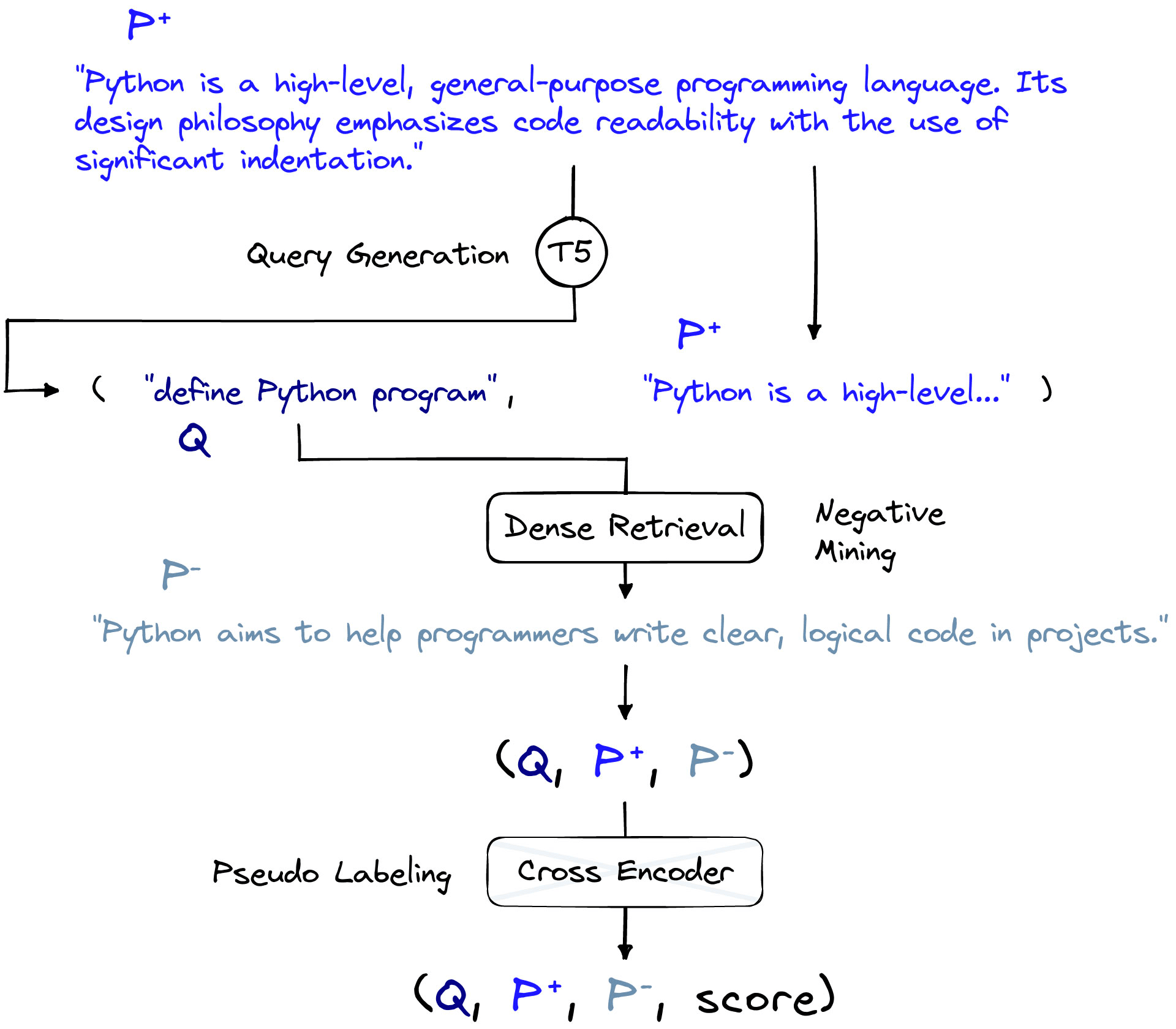
Overview of the GPL process. Beginning with passages P+, we generate queries Q. The passages are indexed and a dense retrieval step is used to find high similarity ‘negative’ passages P-. We then use a cross encoder to produce margin scores.
Each of these steps requires the use of a pre-existing model fine-tuned for each task. The team that introduced GPL also provided models that handle each task. We will discuss these models as we introduce each step and note alternative models where relevant.
1. Query Generation
GPL is perfect for scenarios where we have no labeled data. However, it does require a large amount of unstructured text. That could be text data scraped from web pages, PDF documents, etc. The only requirement is that this text data is in-domain, meaning it is relevant to our particular use case.
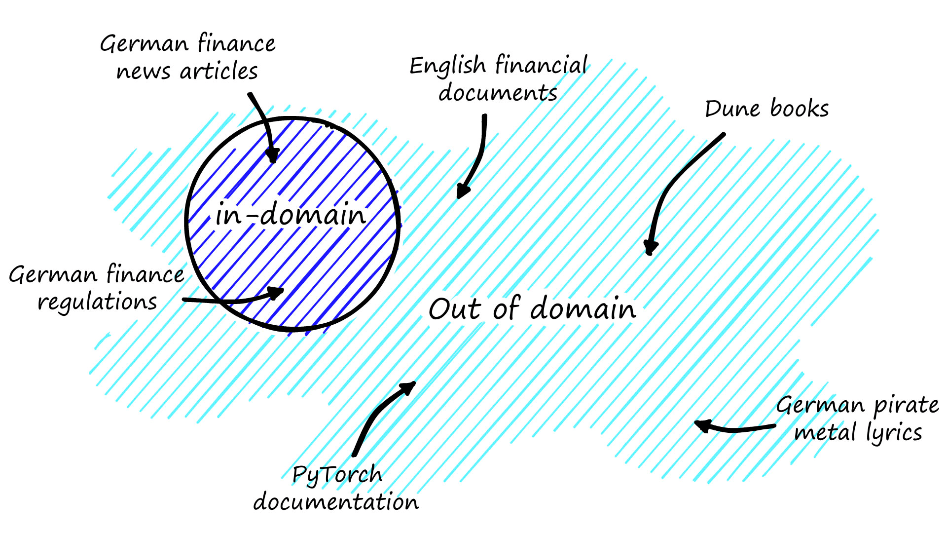
For a target domain of German financial documents, any data that fits the topic and we would expect our model to encounter is in-domain. Anything else is out-of-domain.
In our examples, we will use the CORD-19 dataset. CORD-19 can be downloaded using the script found here. The script will leave many JSON files in a directory called document_parses/pdf_json that we will be using in our query generation step. We will use a generator function called get_text to read in those files.
In[1]:
from pathlib import Path
import json

paths = [str(path) for path in Path('document_parses/pdf_json').glob('*.json')]

def get_text():
    for path in paths:
        with open(path, 'r') as fp:
            doc = json.load(fp)
        # extract the passages of text from each document
        body_text = [line['text'] for line in doc['body_text']]
        # loop through and yield one passage at a time
        for passage in body_text:
            yield passage
If you’ve read our previous chapter on GenQ, this step follows the same query generation process. However, we will outline the process for new readers.
We’re starting with passages of data (the unstructured text data). Generally, these are reasonably long chunks of text, but not always.
In[5]:
passages = get_text()

for i, passage in enumerate(passages):
    print(passage)
    if i == 2: break
Out[5]:
Until recently, seven types of coronaviruses had been reported to cause infections in humans...
An 80-year-old male with a medical history of diabetes, hypertension, dyslipidemia, asthma, coronary...
COVID-19 is a pandemic illness that primarily affects the respiratory system with a wide spectrum of...
Given a passage, we pass it through a query generation T5 model. We can initialize this T5 model using HuggingFace Transformers.
T5 refers to Google’s Text-to-Text Transfer Transformer. We discuss it in more detail in the chapter on GenQ.
In[3]:
from transformers import AutoTokenizer, AutoModelForSeq2SeqLM

model_name = 'doc2query/msmarco-t5-base-v1'

tokenizer = AutoTokenizer.from_pretrained(model_name)
model = AutoModelForSeq2SeqLM.from_pretrained(model_name).cuda()
We are using the doc2query/msmarco-t5-base-v1 model that was trained on a pre-COVID dataset. Nonetheless, when generating queries for COVID-related text the model can produce sensible questions by copying words from the passage text.
With this T5 model, we can begin generating queries that we use to produce synthetic (query, passage) pairs.
In[4]:
for passage in passages:
    break  # just pull a single example

# tokenize the passage
inputs = tokenizer(passage, return_tensors='pt')
# generate three queries
outputs = model.generate(
    input_ids=inputs['input_ids'].cuda(),
    attention_mask=inputs['attention_mask'].cuda(),
    max_length=64,
    do_sample=True,
    top_p=0.95,
    num_return_sequences=3)
In[5]:
print("Paragraph:")
print(passage)

print("\nGenerated Queries:")
for i in range(len(outputs)):
    query = tokenizer.decode(outputs[i], skip_special_tokens=True)
    print(f'{i + 1}: {query}')
Out[5]:
Paragraph:
The surgeons of COVID-19 dedicated hospitals do rarely practice surgery. When ICU patients need mechanical ventilation, percutaneous tracheostomy under endoscopic control is mostly performed...

Generated Queries:
1: why percutaneous tracheostomy
2: what is percutaneous tracheostomy under endoscopic control
3: what is percutaneous tracheostomy
Query generation is not perfect. It can generate noisy, sometimes nonsensical queries. And this is where GPL improved upon GenQ. GenQ relies heavily on these synthetic queries being high-quality with little noise. With GPL, this is not the case as the final cross-encoder step labels the similarity of pairs. Meaning dissimilar pairs are likely to be labeled as such. GenQ does not have any such labeling step.
We now have (query, passage) pairs and can move onto the next step of identifying negative passages.
2. Negative Mining
The (query, passage) pairs we have now are assumed to be positively similar, written as (Q, P+) where the query is Q, and the positive passage is P+.
Suppose we fine-tune our bi-encoder on only these positive matches. In that case, our model will struggle to learn more nuanced differences. A good model must learn to distinguish between similar and dissimilar pairs even where the content of these different pairs is very similar.
To fix this, we perform a negative mining step to find highly similar passages to existing P+ passages. As these new passages will be highly similar but not matches to our query Q, our model will need to learn how to distinguish them from genuine matches P+. We refer to these non-matches as negative passages and are written as P-.
The negative mining process is a retrieval step where, given a query, we return the top_k most similar results. Excluding the positive passage (if returned), we assume all other returned passages are negatives. We then select one of these negative passages at random to become the negative pair for our query.
It may seem counterintuitive at first. Why would we return the most similar passages and train a model to view these as dissimilar?
Yes, those returned results are the most similar passages to our query, but they are not the correct passage for our query. We are, in essence, increasing the similarity gap between the correct passage and all other passages, no matter how similar they may be.
Adding these ‘negative’ training examples (Q, P-) is a common approach used in many bi-encoder fine-tuning methods, including multiple negatives ranking and margin MSE loss (the latter of which we will be using). Using hard negatives in-particular can significantly improve the performance of our models [3].
![The impact on model performance trained on MSMARCO with and without hard negatives. Model training used margin MSE loss. Adapted from [3].](https://www.pinecone.io/_next/image/?url=https%3A%2F%2Fcdn.sanity.io%2Fimages%2Fvr8gru94%2Fproduction%2Fcf65a54c973a99f626a25dfa77ed30f7c4a130f9-1744x1059.png&w=3840&q=75)
The impact on model performance trained on MSMARCO with and without hard negatives. Model training used margin MSE loss. Adapted from [3].
When we later tune our model to identify the difference between these positive and negative passages, we are teaching it to determine what are often very nuanced differences.
With all of that in mind, we do need to understand that only some of the returned passages will be relevant. We will explain how that is handled in the Pseudo-labeling step later.
Moving on to the implementation of negative mining. As before, we need an existing model to embed our passages and create searchable dense vectors. We use the msmarco-distilbert-base-tas-b bi-encoder which was fine-tuned on pre-COVID datasets.
In[1]:
from sentence_transformers import SentenceTransformer

model = SentenceTransformer('msmarco-distilbert-base-tas-b')
model.max_seq_length = 256
model
Out[1]:
SentenceTransformer(
  (0): Transformer({'max_seq_length': 256, 'do_lower_case': False}) with Transformer model: DistilBertModel
  (1): Pooling({'word_embedding_dimension': 768, 'pooling_mode_cls_token': True, 'pooling_mode_mean_tokens': False, 'pooling_mode_max_tokens': False, 'pooling_mode_mean_sqrt_len_tokens': False})
)
In the GPL paper, two retrieval models are used and their results compared. To keep things simple, we will stick with a single model.
We need a vector database to store the passage embeddings. We will use Pinecone as an incredibly easy-to-use service that can scale to the millions of passage embeddings we’d like to search.
In[2]:
import pinecone

with open('secret', 'r') as fp:
    API_KEY = fp.read()  # get api key app.pinecone.io

pinecone.init(
    api_key=API_KEY,
    environment='YOUR_ENV'  # find next to API key in console
)
# create a new genq index if does not already exist
if 'negative-mine' not in pinecone.list_indexes():
    pinecone.create_index(
        'negative-mine',
        dimension=model.get_sentence_embedding_dimension(),
        metric='dotproduct',
        pods=1  # increase for faster mining
    )
# connect
index = pinecone.Index('negative-mine')
We encode our passages, assign unique IDs to each, and then upload the record to Pinecone. As we later need to match these returned vectors back to their original plaintext format, we will create an ID-to-passage mapping to be stored locally.
In[4]:
pair_gen = get_text()  # generator that loads (query, passage) pairs

pairs = []
to_upsert = []
passage_batch = []
id_batch = []
batch_size = 64  # encode and upload size

for i, (query, passage) in enumerate(pairs_gen):
    pairs.append((query, passage))
    # we do this to avoid passage duplication in the vector DB
    if passage not in passage_batch:
        passage_batch.append(passage)
        id_batch.append(str(i))
    # on reaching batch_size, we encode and upsert
    if len(passage_batch) == batch_size:
        embeds = model.encode(passage_batch).tolist()
        # upload to index
        index.upsert(vectors=list(zip(id_batch, embeds)))
        # refresh batches
        passage_batch = []
        id_batch = []

# check number of vectors in the index
index.describe_index_stats()
Out[4]:
100%|██████████| 200/200 [44:31<00:00, 0.07it/s]Out[4]:
{'dimension': 768,
 'index_fullness': 0.0,
'namespaces': {'': {'vector_count': 67840}}}The vector database is set up for us to begin negative mining. We loop through each query, returning 10 of the most similar passages by setting top_k=10.
In[5]:
import random

batch_size = 100
triplets = []

for i in tqdm(range(0, len(pairs), batch_size)):
    # embed queries and query pinecone in batches to minimize network latency
    i_end = min(i+batch_size, len(pairs))
    queries = [pair[0] for pair in pairs[i:i_end]]
    pos_passages = [pair[1] for pair in pairs[i:i_end]]
    # create query embeddings
    query_embs = model.encode(queries, convert_to_tensor=True, show_progress_bar=False)
    # search for top_k most similar passages
    res = index.query(query_embs.tolist(), top_k=10)
    # iterate through queries and find negatives
    for query, pos_passage, query_res in zip(queries, pos_passages, res['results']):
        top_results = query_res['matches']
        # shuffle results so they are in random order
        random.shuffle(top_results)
        for hit in top_results:
            neg_passage = pairs[int(hit['id'])][1]
            # check that we're not just returning the positive passage
            if neg_passage != pos_passage:
                # if not we can add this to our (Q, P+, P-) triplets
                triplets.append(query+'\t'+pos_passage+'\t'+neg_passage)
                break

with open('data/triplets.tsv', 'w', encoding='utf-8') as fp:
    fp.write('\n'.join(triplets))  # save training data to file
Out[5]:
0%| | 0/2000 [00:00<?, ?it/s]In[6]:
# delete the index when done to avoid higher charges (if using multiple pods)
pinecone.delete_index('negative-mine')  # when pods == 1, no charges
We then loop through each set of queries, P+ passages, and their negatively mined results. Next, we shuffle those results and return the first that does not match to our P+ passage, this becomes the P- passage. We write each record to file in the format (Q, P+, P-), ready for the next step.
3. Pseudo-labeling
Pseudo-labeling is the final step in preparing our training data. In this step, we use a cross encoder model to generate similarity scores for both positive and negative pairs.
In[1]:
from sentence_transformers import CrossEncoder

# initialize the cross encoder model first
model = CrossEncoder('cross-encoder/ms-marco-MiniLM-L-6-v2')
model
Out[1]:
<sentence_transformers.cross_encoder.CrossEncoder.CrossEncoder at 0x16e35356ee0>In[2]:
import numpy as np

label_lines = []

# triplets is list of Q, P+, and P- tuples
for line in triplets:
    q, p, n = line
    # predict (Q, P+) and (Q, P-) scores
    p_score = model.predict((q, p))
    n_score = model.predict((q, n))
    # calculate the margin score
    margin = p_score - n_score    # append pairs to label_lines with margin score
    label_lines.append(
        q + '\t' + p + '\t' + n + '\t' + str(margin)
    )

with open("data/triplets_margin.tsv", 'w', encoding='utf-8') as fp:
    fp.write('\n'.join(label_lines))
Given a positive and negative query-passage similarity score (GPL uses dot-product similarity), we then take the difference between both scores to give the margin between both.
We calculate the margin between the two similarity scores to train our bi-encoder model using margin MSE loss, which requires the margin score. After generating these scores, our final data format contains the query, both passages, and the margin score.
This final Pseudo-labeling step is very important in ensuring we have high quality training data. Without it, we would need to assume that all passages returned in the negative mining step are irrelevant to our query and must share the same dissimilarity when contrasted against our positive passages.
In reality this is never the case. Some negative passages are more relevant than others. The authors of GPL split these negative passages into three categories [2].
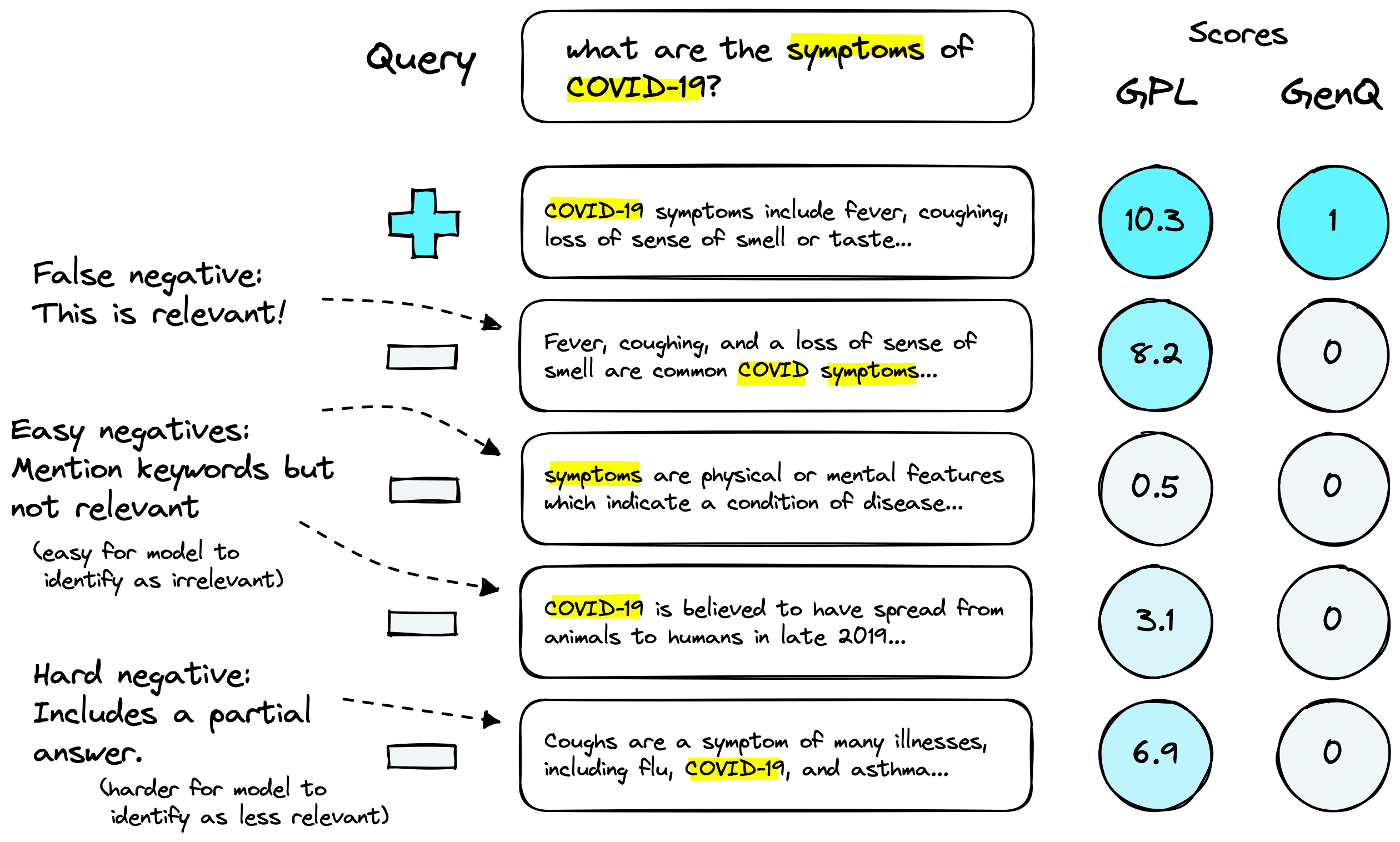
Three categories of negative passages. Whereas previous methods like GenQ that lack the pseudo-labeling step would view passages as either positive 1 or negative 0, GPL can score passages on a more meaningful scale.
We are likely to return a mix of negative passages, from highly relevant to completely irrelevant. Pseudo-labeling allows us to score passages accordingly. Above we can see three negative categories:
- False negatives: we haven’t returned the exact match to our positive passage, but that does not mean we will not return relevant passages (that are in fact not negatives). In this case our cross-encoder will label the passage as relevant, without a cross-encoder this would be marked as irrelevant.
- Easy negatives: these are passages that are loosely connected to the query (such as containing matching keywords) but are not relevant. The cross-encoder should mark these as having low relevance.
- Hard negatives: in this case the passages may be tightly connected to the query, or even contain a partial answer, but still not answer the query. Our cross-encoder should mark these as being more relevant than easy negatives but less so than any positive or false negative passages.
Now that we have our fully prepared data, we can move on to the training portion of GPL.
Training with Margin MSE
The fine-tuning/training portion of GPL is not anything unique or new. It is a tried and tested bi-encoder training process that optimizes with margin MSE loss.
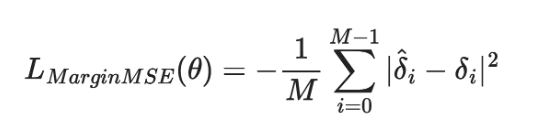
We are looking at the sum of squared errors between the predicted margin 𝛿^i and the true margin 𝛿i for all samples in the training set (from i=0 to i=M-1). We make it a mean squared error by dividing the summed error by the number of samples in the training set M.
Looking back at the generated training data, we have the format (Q, P+, P-, margin). How do these fit into the margin MSE loss function above?
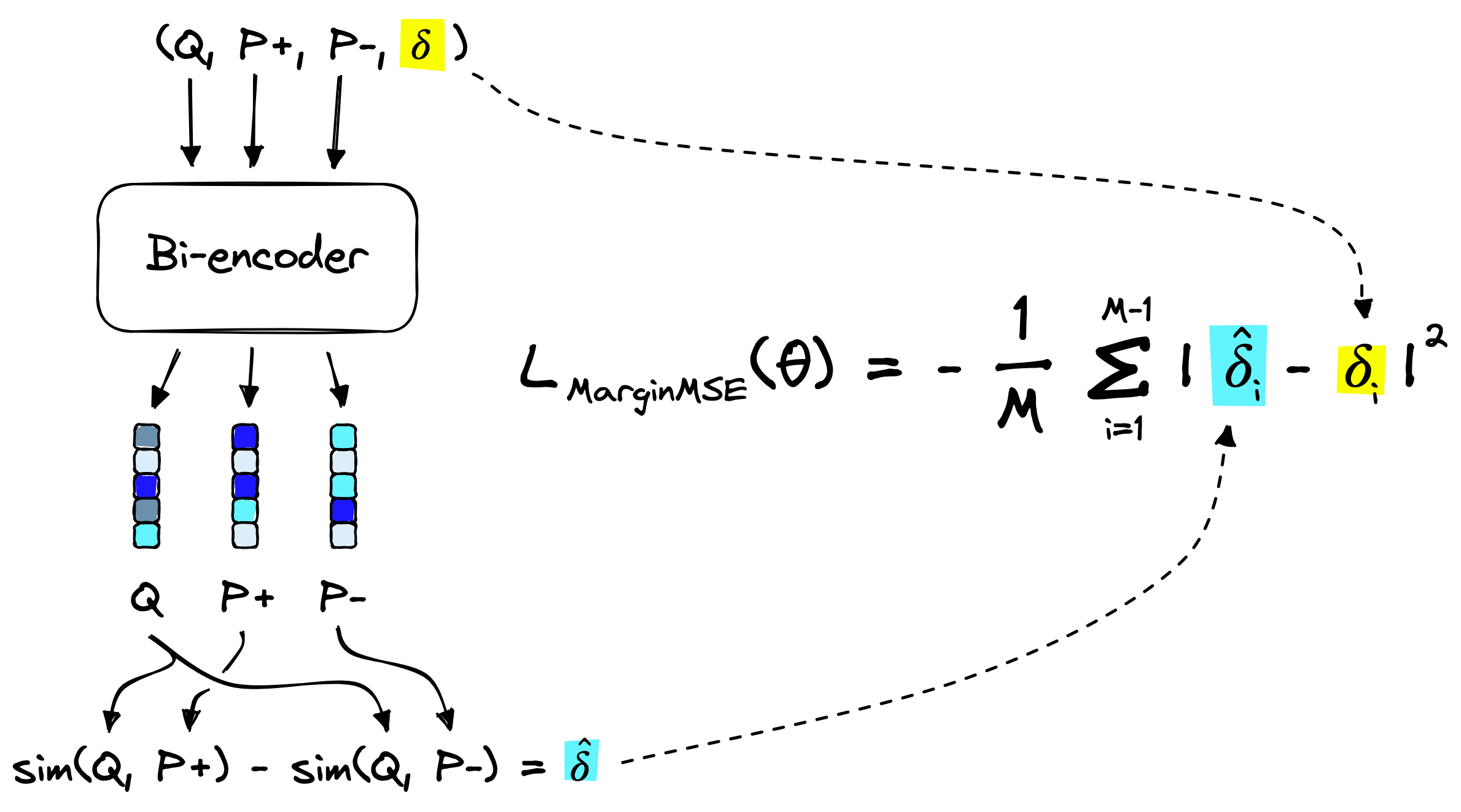
High-level view of (Q, P+, P-) triplets and how they fit into the margin MSE loss function.
The bi-encoder model creates embeddings for the query Q, positive passage *P+, and negative passage P-. We then calculate the dot-product similarity between embeddings for both sim(Q, P+) and sim(Q, P-). These give us the predicted margin:

The true margin 𝛿i has already been calculated by our cross-encoder, it is simply 𝛿i = margin.
We can use the default sentence-transformers methods for fine-tuning models with margin MSE loss. We begin by loading our pairs into a list of InputExample objects.
In[2]:
from sentence_transformers import InputExample

training_data = []

for line in label_lines:
    q, p, n, margin = line.split('\t')
    training_data.append(InputExample(
        texts=[q, p, n],
        label=float(margin)
    ))

len(training_data)
We can see the contents of one of our InputExample objects:
In[3]:
print(f"""
Query: {training_data[0].texts[0]}
Passage +: {training_data[0].texts[1][:100]}...
Passage -: {training_data[0].texts[2][:100]}...
Margin: {training_data[0].label}
""")
Out[3]:
Query: can mutation be introduced to plasmid
Passage +: Mutations were then introduced into the replicon plasmid as described above....
Passage -: It is worth noting that PfSWIB may lead to stage-specific PCD, in the same way as BAF60a of the mamm...
Margin: 17.084930419921875
We use a generic PyTorch DataLoader to load the data into the model during training. One crucial detail is that margin MSE loss works best with large batch sizes. A batch size of 32 or even 64 is a good target, but this does require significant GPU memory and may not be feasible. If that is the case, reduce the batch size until it fits within your hardware restraints.
In[4]:
import torch

torch.cuda.empty_cache()  # clear GPU

batch_size = 32

loader = torch.utils.data.DataLoader(
    training_data, batch_size=batch_size, shuffle=True
)
Next, we initialize a bi-encoder model using the pre-COVID DistilBERT bi-encoder that we used in the negative mining step. It is this model that we are adapting to better understand COVID-19 related language.
In[4]:
from sentence_transformers import SentenceTransformer

model = SentenceTransformer('msmarco-distilbert-base-tas-b')
model.max_seq_length = 256
model
Out[4]:
SentenceTransformer(
  (0): Transformer({'max_seq_length': 256, 'do_lower_case': False}) with Transformer model: DistilBertModel
  (1): Pooling({'word_embedding_dimension': 768, 'pooling_mode_cls_token': True, 'pooling_mode_mean_tokens': False, 'pooling_mode_max_tokens': False, 'pooling_mode_mean_sqrt_len_tokens': False})
)
We’re ready to initialize the margin MSE loss that will optimize the model later.
In[6]:
from sentence_transformers import losses

loss = losses.MarginMSELoss(model)
With that, we’re finally ready to begin fine-tuning our model. We used a single epoch, with a training set of 600K samples this is a large number of steps. It was found that GPL performance tends to stop improving after around 100K steps [2]. However, this will vary by dataset.
![NDCG@10% performance for zero-shot (not adapted), GPL fine-tuned, and GPL fine-tuned + TSDAE pre-trained models. GPL fine-tuning using a model that had previously been pretrained using TSDAE demonstrates consistently better performance. Model performance seems to level-out after 100K training steps. Visual adapted from [2].](https://www.pinecone.io/_next/image/?url=https%3A%2F%2Fcdn.sanity.io%2Fimages%2Fvr8gru94%2Fproduction%2F32dca390f3667aad12274e4d8f9baae6a205b54b-1744x1139.png&w=3840&q=75)
NDCG@10% performance for zero-shot (not adapted), GPL fine-tuned, and GPL fine-tuned + TSDAE pre-trained models. GPL fine-tuning using a model that had previously been pretrained using TSDAE demonstrates consistently better performance. Model performance seems to level-out after 100K training steps. Visual adapted from [2].
In[8]:
from sentence_transformers import SentenceTransformer

model = SentenceTransformer('msmarco-distilbert-base-tas-b-covid')
Once training is complete, we will find all of our model files in the msmarco-distilbert-base-tas-b-covid directory. To use our model in the future, we simply load it from the same directory using sentence-transformers.
In[8]:
from sentence_transformers import SentenceTransformer

model = SentenceTransformer('msmarco-distilbert-base-tas-b-covid')
If you’d like to use the model trained in this article, you can specify the model name pinecone/msmarco-distilbert-base-tas-b-covid.
Now let’s return to the COVID-19 queries we asked the initial model (without GPL adaptation).
Out[14]:
Query: How is COVID-19 transmitted
101.72	Corona is transmitted via the air
101.57	Ebola is transmitted via direct contact with blood
100.58	HIV is transmitted via sex or sharing needles

Query: what is the latest named variant of corona
99.32	people keep drinking corona lager
98.77	the omicron variant of SARS-CoV-2
90.97	COVID-19 is an illness caused by a virus

Query: What are the symptoms of COVID-19?
99.37	common Corona symptoms include a high temperature, cough, and fatigue
98.75	common Flu symptoms include a high temperature, aching body, and fatigue
97.51	symptoms are a physical or mental features which indicate a condition of disease

Query: How will most people identify that they have contracted the coronavirus
97.69	after drinking too many bottles of corona beer most people are hungover
97.35	the most common COVID-19 symptoms include a high temperature, cough, and fatigue
93.53	common symptoms of flu include a high temperature, aching, and exhaustion
As before we are asking four questions, each of which has three possible passages. Our model is tasked with scoring the similarity of each passage, the goal is to return COVID-19 related sentences higher than any other sentences.
We can see that this has worked for two of our queries. For the two queries it performs worse on, it looks like our GPL trained model is confusing the drink Corona with “corona” in the context of COVID-19.
What we can do is try and fine-tune our model for more epochs, if we try again with a model trained for 10 epochs we get more promising results.
In[15]:
show_examples(gpl_model10)Out[15]:
Query: How is COVID-19 transmitted
98.21	Corona is transmitted via the air
96.15	Ebola is transmitted via direct contact with blood
94.77	HIV is transmitted via sex or sharing needles

Query: what is the latest named variant of corona
93.19	the omicron variant of SARS-CoV-2
93.10	people keep drinking corona lager
86.33	COVID-19 is an illness caused by a virus

Query: What are the symptoms of COVID-19?
95.02	common Corona symptoms include a high temperature, cough, and fatigue
94.21	common Flu symptoms include a high temperature, aching body, and fatigue
93.02	symptoms are a physical or mental features which indicate a condition of disease

Query: How will most people identify that they have contracted the coronavirus
91.62	the most common COVID-19 symptoms include a high temperature, cough, and fatigue
91.36	after drinking too many bottles of corona beer most people are hungover
87.99	common symptoms of flu include a high temperature, aching, and exhaustion
Now we see much better results and our model is more easily differentiating between the Corona beer, and COVID-19.
A Simpler Approach
We’ve worked through a lot of theory and code to understand GPL, and hopefully, it is now much clearer. However, we don’t need to work through all of that to apply GPL. It is much easier when using the official GPL library.
Doing the same as we did before requires little more than a few lines of code. To start, we first pip install gpl. Our input data must use the BeIR data format, a single JSON lines (.jsonl) file called corpus.jsonl. Each sample in the file will look like this:
{
    "_id": "string ID value",
    "title": "string, can be empty",
    "text": "string, the primary content of the sample, like a paragraph of text",
    "metadata": {
        "key1": "metadata is a dictionary containing additional info",
        "key2": "key-value pairs do not need to be str-str",
        "for example": 1337,
        "don't forget": "the dictionary can be empty too"
    }
}
Our CORD-19 dataset is not initially in the correct format, so we must first reformat it.
from tqdm.auto import tqdm
import json
import os

# create directory if needed
if not os.path.exists('./cord_data'):
os.mkdir('./cord_data')

id_count = 0

with open('./cord_data/corpus.jsonl', 'w') as jsonl:
    for path in tqdm(paths):
        # read each json file in the CORD-19 pdf_json directory
        with open(path, 'r') as fp:
            doc = json.load(fp)
        # extract the passages of text from each document
        for line in doc['body_text']:
            line = {
                '_id': str(id_count),
                'title': "",
                'text': line['text'].replace('\n', ' '),
                'metadata': doc['metadata']
            }
            id_count += 1
    # iteratively write lines to the JSON lines corpus.jsonl file
    jsonl.write(json.dumps(line)+'\n')
Now we will have a new corpus.jsonl file in the cord_data directory. The first sample from the newly formatted CORD-19 dataset looks similar to this:
{
    "_id": "0",
    "title": "",
    "text": "Digital technologies have provided support in diverse policy...",
    "metadata": {
        "title": "Students' Acceptance of Technology...",
        "authors": [
            {"first": "Pilar", "last": "Lacasa"},
            {"first": "Juan", "last": "Nieto"},
            ...
        ]
    }
}
With that newly formatted dataset, we can run the whole GPL data generation and fine-tuning process with a single, slightly lengthy function call.
import gpl

gpl.train(
    path_to_generated_data='./cord_data',
    base_ckpt='distilbert-base-uncased',
    batch_size_gpl=16,
    gpl_steps=140_000,
    output_dir='./output/cord_model',
    generator='BeIR/query-gen-msmarco-t5-base-v1',
    retrievers=[
        'msmarco-distilbert-base-v3',
        'msmarco-MiniLM-L-6-v3'
    ],
    cross_encoder='cross-encoder/ms-marco-MiniLM-L-6-v2',
    qgen_prefix='qgen',
    do_evaluation=False
)
Let’s break all of this down. We have:
path_to_generated_data- the directory containing corpus.jsonl.base_ckpt- the starting point of the bi-encoder model that we will be fine-tuning.batch_size_gpl- batch size for the margin MSE loss fine-tuning step.gpl_steps- number of training steps to run for the MSE margin loss fine-tuning.output_dir- where to save the fine-tuned bi-encoder model.generator- the query generation model.retrievers- a list of retriever models to use in the negative mining step.cross_encoder- the cross encoder model used for pseudo-labeling.qgen_prefix- the query generation data files prefix.do_evaluation- whether to evaluate the model on an evaluation dataset requires an evaluation set to be provided.
After running this, which can take some time, we have a bi-encoder fine-tuned using GPL on nothing more than the passages of text passed from the ./cord_data/corpus.jsonl file.
Using the GPL library is a great way to apply unsupervised learning. When compared to our more in-depth process, it is much simpler. The one downside is that the negative mining step uses exhaustive search. This type of search is no problem for smaller corpora but becomes slow for larger datasets (100K–1M+) and, depending on your hardware, impossible for anything too large to be stored in memory.
That’s it for this chapter on Generative Pseudo-Labeling (GPL). Using this impressive approach, we can fine-tune new or existing models in domains that were previously inaccessible due to little or no labeled data.
The research on unsupervised training methods for bi-encoder models continues to progress. GPL is the latest in a series of techniques that extends the performance of these exciting models trained without labeled data.
What is possible with GPL is impressive. Perhaps even more exciting is the possibility of further improvements to GPL or completely new methods that take the performance of these unsupervised training methods to even greater heights.
References
[1] T. Berners-Lee, M. Fischetti, Weaving the Web, The Original Design and Ultimate Destiny of the World Wide Web by Its Inventor (1999)
[2] K. Wang, et al., GPL: Generative Pseudo Labeling for Unsupervised Domain Adaptation of Dense Retrieval
[3] Y. Qu, et al., RocketQA: An Optimized Training Approach to Dense Passage Retrieval for Open-Domain Question Answering (2021), NAACL
Was this article helpful?